阿里巴巴推出的Qwen 3是继DeepSeek之后当前最优秀的开源混合专家（MoE）AI模型，在推理、编程、数学和语言处理方面表现卓越。其顶级版本在MMLU-Pro、LiveCodeBench和AIME等关键基准测试中名列前茅。若读者对LLM知识储备不多，但是又想短时间想了解MOE全貌，这篇文章最适合入门阅读和体会。

        本文章将从零理解和构建Qwen-3 MoE，让读者能够更加清晰理解，来源：

Building Qwen-3 MoE from Scratch Without OOP in Python

Owner avatar qwen3-MoE-from-scratch

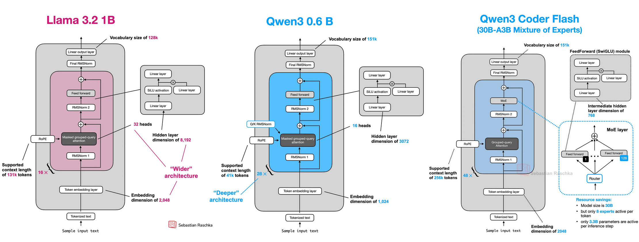
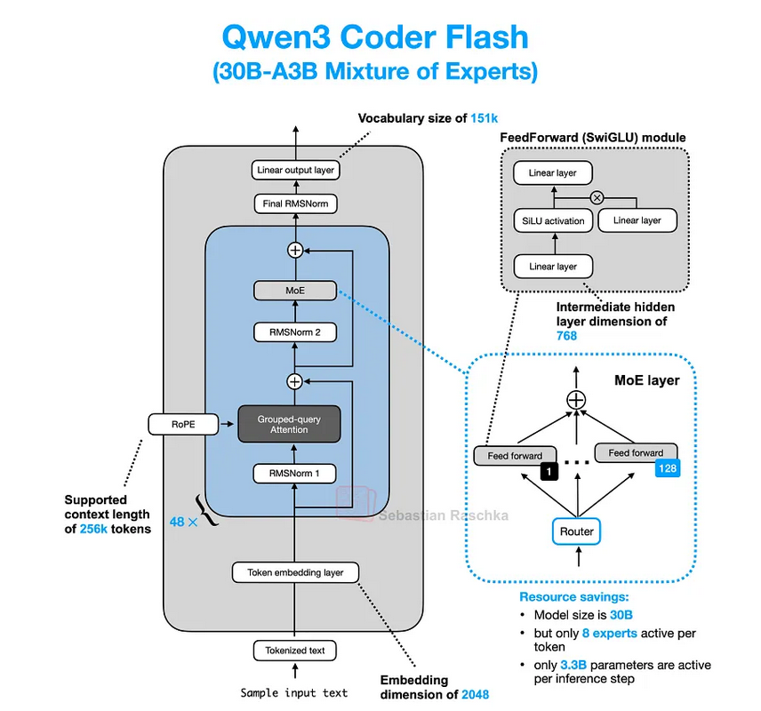
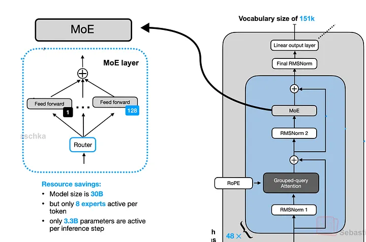
        Qwen 3采用混合专家（MoE）架构构建，每次查询仅激活其2350亿参数中的一个子集，在保证质量的同时实现高效运行。该模型还支持高达128K token的上下文长度，兼容119种语言，并引入了双模式设计——"思考模式"与"非思考模式"，在深度推理与快速响应之间实现平衡。

1 理解Qwen 3混合专家（MoE）架构

        首先，让我们以具备一定技术基础的学习者视角来理解Qwen的MoE架构，然后通过"the cat sat"（猫坐着）这个具体示例，追踪其在该架构中的处理流程，从而获得清晰认知。

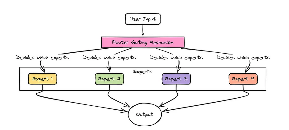
        想象你接手了一项极其艰巨的工作。与其雇一个样样都懂一点的全能型员工，不如组建一支专家团队——每位专家都精通某个特定领域（比如电工、水管工、油漆工）。你还会聘请一位经理，由他根据当前任务指派合适的专家来处理。

        AI模型中的MoE（混合专家）机制正是基于这个理念。不同于让一个庞大的神经网络试图学习所有知识，MoE层采用以下结构：

1. A Team of “Experts”: 由多个小型专业化神经网络组成（通常是简单的前馈网络或MLP多层感知机）。每个专家可能擅长处理某类特定信息或模式。
2. A “Router” (The Manager): 这是另一个小型网络，其职责是分析输入数据（比如某个单词或词片段），并判断当前最适合处理该数据的专家组合。

#########假设我们的模型正在处理句子："The cat sat."

​​（2）分词处理​​：首先，我们将句子拆分为若干片段（即标记/token）："The"、"cat"、"sat"。

（3）Router 收标记​​：MoE 层接收到标记 ​​"cat"​​（它会被表示为一组数字，即嵌入向量/embedding vector）。此时，​​Router​​ 会分析这个 ​​"cat" 向量​​。

（4）Router做出选择​​：假设有 4 个专家（E1、E2、E3、E4）。路由会判断哪些专家最适合处理 ​​"cat"​​。

​​（5）可能的决策​​：比如，它认为 ​​E2​​（或许擅长处理名词？）和 ​​E4​​（或许擅长处理动物相关概念？）是最合适的选择。于是，它会为这些专家分配分数或"权重"（例如，E2 得 70% 权重，E4 得 30% 权重）。

        ​"cat" 向量仅被发送给专家 E2 和 E4​​。专家 E1 和 E3 在处理这个标记时无需工作，从而节省了计算资源！

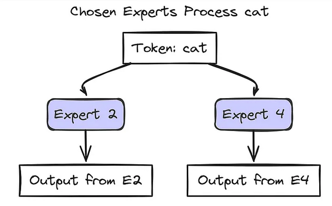
        我们通过路由分配的权重合并所选专家的输出结果：最终输出 = (0.7 × Output_E2) + (0.3 × Output_E4)​​；这个 ​​Final_Output​​ 就是 MoE 层针对标记 ​​"cat"​​ 最终传递的结果。而序列中的每个标记都会经历这样的处理流程！不同标记可能会被路由到不同的专家组合。

        因此，当模型处理类似 ​​"The cat sat."​​ 这样的文本时，整体处理流程如下：

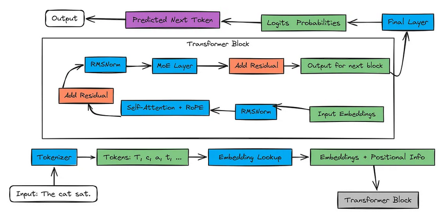
        输入文本进入分词器（常用有BPE）。分词器生成数字形式的标记ID。嵌入层将这些ID转换为有意义的数字向量（即嵌入向量），并添加位置信息（后续在注意力机制中通过RoPE实现）。

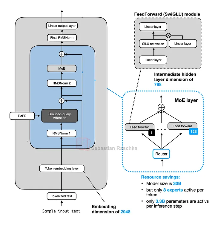
        这些向量会经过多个Transformer模块。每个模块包含：（a）自注意力机制；（b）Router 分配，混合专家层；（c）归一化（RMSNorm）和残差连接有助于模型学习；

        最后一个模块的输出会传入最终层。该层为词汇表中每一个可能的下一个标记生成对数几率（即得分）。我们将这些对数几率转换为概率，并预测下一个标记。

        现在我们已经了解了混合专家（MoE）在整个流程中的位置，接下来让我们深入探究每个AI模型的更小组成部分。

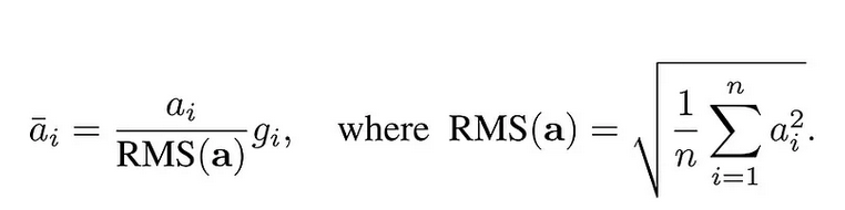
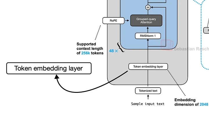
1.1 采用RMSNorm进行预归一化

        在每个Transformer子层（注意力层或前馈层）之前应用RMSNorm（均方根归一化）。它根据输入的均方根进行缩放，但不减去均值（与LayerNorm不同）。这有助于稳定训练，并在早期保持重要信号的强度，就像在深入学习教科书之前先复习关键章节一样，相关参考论文《Root Mean Square Layer Normalization》。

对比：层归一化（layernorm）在计算均值和方差时只考虑单个样本的所有特征：

这里 是参数， 是单个样本的均值， 是单个样本的方差，分别是缩放和偏移系数。

1.2 SwiGLU 激活函数

        SwiGLU（Swish激活函数+门控线性单元）增强了模型突出重要特征的能力。它采用基于Swish激活函数的门控机制，有助于控制哪些信息能够通过。

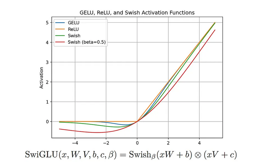
        可以把它想象成一个智能荧光笔，在处理过程中让关键部分更加突出。该机制最早在PaLM模型中引入，如今已在LLaMA 3和Qwen 3等模型中应用以提升性能。

Swish 函数的数学表达式为：

是输入值，是sigmoid函数， 是可学习参数（通常初始化为 1，后续可训练调整）；该函数结合了ReLU的线性响应特性和Sigmoid的平滑特性。

关于SwiGLU的更多细节，可参阅相关《GLU Variants Improve Transformer》论文。

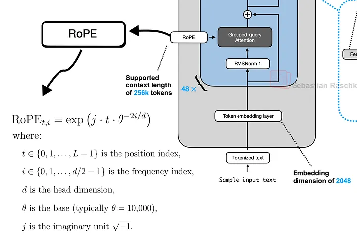
1.3 旋转位置编码（RoPE）

        RoPE（旋转位置编码）利用带有旋转特性的正弦函数对词元（token）的位置进行编码，使得嵌入向量能够通过“旋转”来反映相对位置关系。

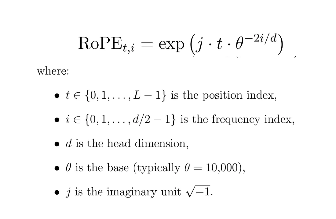
        与固定位置嵌入不同，RoPE 支持更长的上下文，并且能更好地泛化到未见过的位置。想象一群学生围成一个圆圈移动——他们的绝对位置在变化，但彼此之间的相对距离保持不变。这种方式帮助模型更灵活地追踪词语的顺序。

1.4 Byte Pair Encoding (BPE)

        BPE（字节对编码）通过不断合并高频字符对（如“th”“ing”）来构建词元（token），从而使模型能够更高效地处理不常见或新出现的词汇。

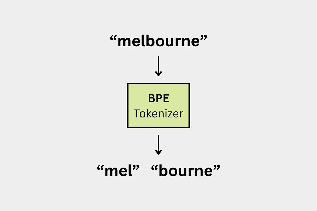
        Qwen 3 使用的是 BPE（字节对编码），它倾向于保留完整已知的单词（例如，如果“hugging”在词表中，就会作为一个整体存在）。而 LLaMA 3 使用的是 SentencePiece 实现的 BPE，这种实现可能会把同一个单词拆分成多个部分（比如拆成“hug” + “ging”）。这一差异会影响到分词速度，也会影响模型对文本的理解方式。

2 阶段设置

        将使用少量 Python 库，但建议提前安装这些库，以避免运行时出现“找不到模块（no module found）”的错误。

# Download Required modules
pip install sentencepiece tiktoken torch matplotlib huggingface_hub tokenizers safetensors

        在安装完所需的库之后，我们需要下载本指南中将用到的 Qwen 3 模型架构的权重文件和配置文件。

        我们选用的是一个较小规模的 Qwen 3 MoE（混合专家）版本，该版本包含两个专家网络，每个专家的参数量为 0.80 亿（0.8B）。这些必要的文件构成了 Qwen 3 模型架构的核心部分。下载这些文件有两种方式可供选择。

选项1：ModelScope下载

        如果没有科学工具，首先考虑在ModelScope寻找开源版本：huihui-ai/Huihui-MoE-0.8B-2E

pip install modelscope
modelscope download huihui-ai/Huihui-MoE-0.8B-2E --local_dir ./Huihui-MoE-0.8B-2E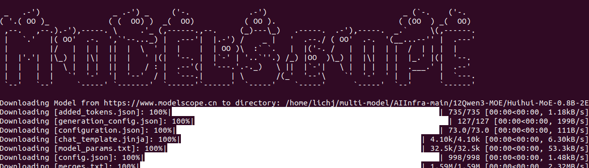

选项 2：镜像下载（适合linux/macOS）

export HF_ENDPOINT=https://hf-mirror.com  # Linux/macOS
pip install "huggingface_hub[cli]"
# 下载一个文件
huggingface-cli download huihui-ai/Huihui-MoE-0.8B-2E --local-dir ./Huihui-MoE-0.8B-2E

        Huihui-MoE-0.8B-2E​​ 是由 huihui.ai 开发的一款基于 ​​Mixture of Experts（混合专家，简称 MoE）​​ 架构的语言模型，其基础模型为 ​​Qwen/Qwen3-0.6B​​。该模型在标准 Transformer 架构的基础上进行了改进，将传统的多层感知机（MLP）层替换为包含 ​​2 个专家网络（experts）​​ 的 MoE 层，在保证高性能的同时实现了高效的推理。此模型专为自然语言处理任务设计，适用于 ​​文本生成、问答系统以及对话应用​​ 等多种场景。目前，​​Huihui-MoE-0.8B-2E 是参数量最小的 MoE 模型之一​​，并且具备良好的可扩展性，未来可以根据需求增加更多的专家网络。该模型 ​​尚未经过特定任务的微调（fine-tuning）​​，但你可以根据自身需求对其进行微调，以适配具体应用场景。如果你 ​​不进行微调​​，也可以像使用原始模型 ​​Qwen/Qwen3-0.6B​​ 一样直接调用和使用该模型。

选项 3：手动下载

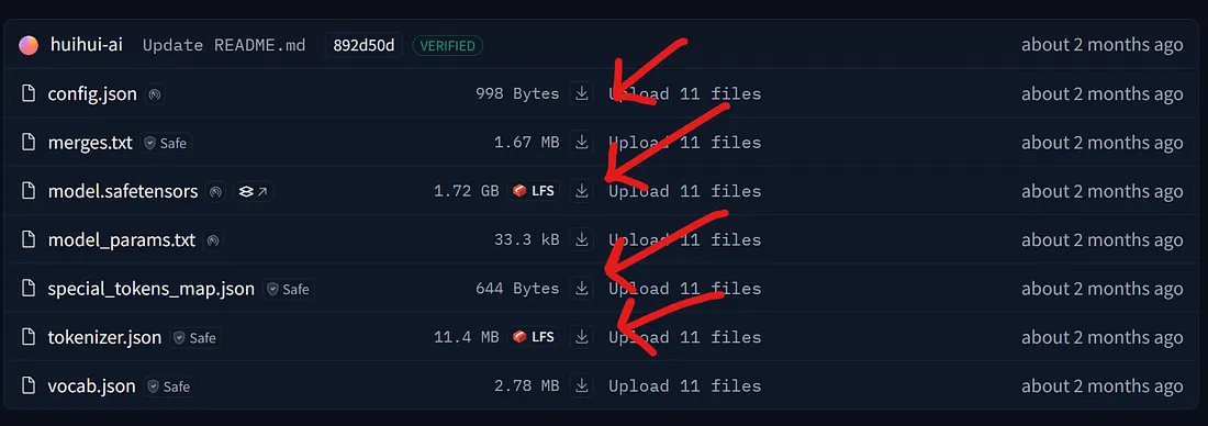
        前往 Qwen-0.8B-2E 的 Hugging Face（HF）模型目录，手动下载以下四个文件。

选项 4：Coding

       可以使用 ​​huggingface_hub​​ 提供的 snapshot downloader 模块，来下载 Qwen 3 MoE 模型在 Hugging Face 上的整个仓库内容。接下来，我们就采用这种方法进行下载。

# Import tqdm for progress bars and snapshot_download for downloading model files
from tqdm import tqdm
from huggingface_hub import snapshot_download

# Define the Hugging Face repository ID and the local directory to save the files
repo_id = "huihui-ai/Huihui-MoE-0.8B-2E"
local_dir = "Huihui-MoE-0.8B-2E"

# Download the model snapshot from Hugging Face, excluding .bin files
# This will fetch config, tokenizer, and safetensors weights only
snapshot_download(
    repo_id=repo_id,
    local_dir=local_dir,
    ignore_patterns=["*.bin"],      # Skip large .bin files, only get safetensors
    tqdm_class=tqdm                # Use standard tqdm for progress bar
)

所有文件下载完成后，我们需要导入本教程中将会用到的各个库。.

3 为什么要模型权重？

        因为我们目标是 ​​精准复现 Qwen 3 MoE 模型​​，这意味着当我们输入一段文本时，模型必须能够给出有意义的输出。举个例子，如果输入是：“the color of the sun is?”（太阳是什么颜色的？），那么期望的输出就应该是：“white”（白色）。要实现这样的效果，就需要在大规模数据集上对大语言模型（LLM）进行训练，而这需要非常强大的计算资源，在个人或小团队环境下通常是难以实现的。

        不过，​​阿里巴巴已经公开发布了 Qwen 3 的模型架构文件​​，更专业一点的说法就是，他们开放了 ​​预训练模型权重（pretrained weights）​​ 供大家使用。我们刚才已经下载了这些文件，这意味着我们现在可以 ​​复现 Qwen 3 的模型架构，而无需从头开始训练，也不用准备大规模的数据集​​。一切基础已经搭建好了，我们只需要把各个组件放在正确的位置上即可。

---

tokenizer.json 文件说明: Qwen 3 使用的是 ​​字节对编码（Byte Pair Encoding，简称 BPE）​​，这是一种主流的词元（token）构建方法。值得一提的是，AI 研究者 Andrej Karpathy 对 BPE 有一个非常清晰简洁的实现minbpe，值得参考。

# This file contains the vocabulary, merge rules, and configuration.
tokenizer_path = Path("Huihui-MoE-0.8B-2E/tokenizer.json")

# The Tokenizer.from_file() method is the standard way to load tokenizers
# from the Hugging Face ecosystem.
tokenizer = Tokenizer.from_file(str(tokenizer_path))

# We can also load them from the special_tokens_map.json for confirmation
with open("Huihui-MoE-0.8B-2E/special_tokens_map.json", "r") as f:
    special_tokens_map = json.load(f)
    print(f"Special tokens from file: {special_tokens_map}")


#### OUTPUT ####

Special tokens from file: {
'additional_special_tokens': ['<|im_start|>', 
'<|im_end|>', '<|object_ref_start|>', '<|object_ref_end|>', '<|box_start|>'
...
}

        这些 Special tokens 将用于包裹我们的提示词（prompt），从而指导 Qwen 3 模型架构如何对我们的查询（query）做出回应。

# We'll follow the encode -> decode pattern to ensure it works correctly.
prompt = "The only thing I know is that I know"

# .encode() returns an Encoding object, we access the token IDs via .ids
encoded = tokenizer.encode(prompt)
print(f"\nOriginal prompt: '{prompt}'")
print(f"Encoded token IDs: {encoded.ids}")

# .decode() converts the token IDs back to a string.
decoded = tokenizer.decode(encoded.ids)
print(f"Decoded back to text: '{decoded}'")

# Verify the vocabulary size
vocab_size = tokenizer.get_vocab_size()
print(f"\nTokenizer vocabulary size: {vocab_size}")


#### OUTPUT ####
Original prompt: 'The only thing I know is that I know'
Encoded token IDs: [785, 1172, 3166, 358, 1414, 374, 429, 358, 1414]
Decoded back to text: 'The only thing I know is that I know'
Tokenizer vocabulary size: 151669

        词汇表大小表示的是训练数据中 ​​不同字符（或词元）的总数量​​。该分词器属于 ​​字典（词典）类型​​。

# Get the vocabulary as a dictionary: {token_string: token_id}
vocab = tokenizer.get_vocab()

# Display a slice of the vocabulary for inspection (tokens 5600 to 5609)
sample_vocab_slice = list(vocab.items())[5600:5610]
sample_vocab_slice

#### OUTPUT ####
[('íĮIJ', 129382),
 ('ĠBrands', 54232),
 ('Ġincorporates', 51824),
 ('à¸ŀระราà¸Ĭ', 132851),
 ('ĉResource', 79487),
 ('ĠĠĠĠĉĠ', 80840),
 ('hover', 17583),
 ('Movement', 38050),
 ('解åĨ³äºĨ', 105826),
 ('ĠonBackPressed', 70609)]

        当我们从中打印10个随机项目时，您将看到使用BPE算法形成的字符串。键表示BPE训练中的字节序列，而值表示基于频率的合并排名。在 BPE（字节对编码）算法中，​​合并排名 的数值越小，表示该字节对的 ​​合并优先级越高​​。

config.json — 包含各种参数，例如:

# Define the path to the configuration file.
config_path = Path("Huihui-MoE-0.8B-2E/config.json")

# Open and load the JSON file into a Python dictionary.
with open(config_path, "r") as f:
    config = json.load(f)

# Print the configuration to see all the parameters.
# This gives us a complete overview of the model we're about to build.
print(json.dumps(config, indent=4))


#### OUTPUT ####
{
    "architectures": [
        "Qwen3MoeForCausalLM"
    ],
    "attention_bias": false,
    "attention_dropout": 0.0,
    "bos_token_id": 151643,
    "decoder_sparse_step": 1,
    "eos_token_id": 151645,
    "head_dim": 128,
    "hidden_act": "silu",
    ...
    "transformers_version": "4.52.4",
    "use_cache": true,
    "use_sliding_window": false,
    "vocab_size": 151936
}

        这些参数值将通过明确指定头数（heads）、嵌入向量的维度、专家数量等细节，帮助我们复现 Qwen-3 的架构。让我们将这些值保存下来，以便后续使用。

# --- Main Architecture Parameters ---
# Extract model hyperparameters from the config dictionary.

# Embedding dimension (hidden size of the model)
dim = config["hidden_size"]
# Number of transformer layers
n_layers = config["num_hidden_layers"]
# Number of attention heads
n_heads = config["num_attention_heads"]
# Number of key/value heads (for grouped-query attention)
n_kv_heads = config["num_key_value_heads"]
# Vocabulary size
vocab_size = config["vocab_size"]
# RMSNorm epsilon value for numerical stability
norm_eps = config["rms_norm_eps"]
# Rotary positional embedding theta parameter
rope_theta = torch.tensor(config["rope_theta"])
# Dimension of each attention head
head_dim = config["head_dim"]  # For attention calculations

# --- Mixture-of-Experts (MoE) Specific Parameters ---
# Number of experts in the MoE layer
num_experts = config["num_experts"]
# Number of experts selected per token by the router
num_experts_per_tok = config["num_experts_per_tok"]
# Intermediate size of the MoE feed-forward network
moe_intermediate_size = config["moe_intermediate_size"]

model.safetensors — 包含了 Qwen 0.8B 2Experts 模型学到的参数（即权重）。这些参数记录了模型如何理解和处理语言的信息，例如它是如何表示词元（tokens）、计算注意力（attention）、进行专家选择（experts selection）以及归一化输出（normalize its outputs）的。

# Define the path to the model weights file
model_weights_path = Path("Huihui-MoE-0.8B-2E/model.safetensors")

# Load the weights into a dictionary; each key is a layer/parameter name, and each value is a torch tensor
model_weights = load_file(model_weights_path)

# Inspect the loaded weights: print the first 20 layer names to confirm successful loading
print("First 20 keys in model_weights:")
print(json.dumps(list(model_weights.keys())[:20], indent=4))


#### OUTPUT ####
[
    "model.embed_tokens.weight",
    "model.layers.0.input_layernorm.weight",
    "model.layers.0.mlp.experts.0.down_proj.weight",
    "model.layers.0.mlp.experts.0.gate_proj.weight",
    "model.layers.0.mlp.experts.0.up_proj.weight",
    "model.layers.0.mlp.experts.1.down_proj.weight",
    ...
    "model.layers.1.mlp.experts.0.gate_proj.weight",
    "model.layers.1.mlp.experts.0.up_proj.weight"
    ...
]

        如果您熟悉 Transformer 架构，那么您应该已经了解过查询矩阵（query matrix）、键矩阵（key matrix）等相关概念。稍后，我们将利用这些层（layers）和权重（weights），在 Qwen 3 MoE 的架构中构建类似的矩阵，并加入混合专家（MoE，Mixture of Experts）组件。

        现在，我们已经拥有了分词器（tokenizer）、包含权重的架构模型（architecture model），以及配置参数（configuration parameters），接下来就让我们从零开始编写属于我们自己的 Qwen 3 MoE 模型吧。

4 Tokenized Text

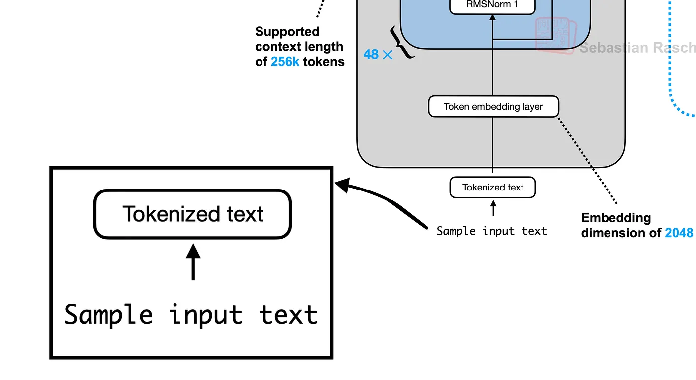
        第一步是将我们的输入文本转换为词元（tokens）。Qwen 3 使用一种特定的对话模板，并包含特殊词元（special tokens），例如 <|im_start|> 和 <|im_end|>，用于构建对话结构。这有助于模型区分用户的问题（queries）与模型自身的回复（responses）。

# Our sample user prompt
prompt = "The only thing I know is that I know"

# Get token IDs for special tokens and template components
im_start_id = tokenizer.token_to_id("<|im_start|>")
im_end_id = tokenizer.token_to_id("<|im_end|>")
newline_id = tokenizer.encode("\n").ids[0]
user_ids = tokenizer.encode("user").ids
assistant_ids = tokenizer.encode("assistant").ids
prompt_ids = tokenizer.encode(prompt).ids

# Manually construct the full prompt using the chat template:
# <|im_start|>user\n{prompt}<|im_end|>\n<|im_start|>assistant\n
prefix_ids = [im_start_id] + user_ids + [newline_id]
suffix_ids = [im_end_id, newline_id, im_start_id] + assistant_ids + [newline_id]
tokens_list = prefix_ids + prompt_ids + suffix_ids

# Convert the list of token IDs into a PyTorch tensor
tokens = torch.tensor(tokens_list)

print(f"Final combined token IDs: {tokens}")

# Decode for verification
prompt_split_as_tokens = [tokenizer.decode([token.item()]) for token in tokens]
print(f"\nPrompt split into tokens: {prompt_split_as_tokens}")


#### OUTPUT ####
Final combined token IDs: tensor([151644,    872,  ... , 8])
Prompt split into tokens: ['', 'user', '\n', 'The', ..., '\n']
#### OUTPUT ####

        现在，我们已经将提示词（prompt）转换成了一个由 17 个词元（tokens）组成的结构化列表，可以输入给模型进行处理了。

5 创建 Token Embedding Layer

       embedding 是一个稠密向量，用于在高维空间中表示词元（token）的语义信息。我们需要将包含 17 个词元的输入向量，转换成一个形状为 [17, 1024] 的张量，其中 1024（即 dim，代表 embedding 维度）就是嵌入向量的维度。

# Initialize the embedding layer with the correct size
embedding_layer = nn.Embedding(vocab_size, dim)
# Load the pre-trained weights into our layer
embedding_layer.weight.data.copy_(model_weights["model.embed_tokens.weight"])

# Pass our tokens through the layer to get their embeddings
token_embeddings_unnormalized = embedding_layer(tokens).to(torch.bfloat16)

# Verify the shape
print("Shape of the token embeddings:", token_embeddings_unnormalized.shape)


#### OUTPUT ####
Shape of the token embeddings: torch.Size([17, 1024])
#### OUTPUT ####

        这些嵌入向量目前尚未经过归一化处理，如果不进行归一化，将会对模型产生严重影响。在下一节中，我们将对输入向量执行归一化操作。

6 使用 RMSNorm 进行归一化

        将定义 rms_norm 函数，该函数基于输入向量的均方根（Root Mean Square，RMS）值对其进行缩放。这一步是我们 Transformer 层中的第一个预归一化（pre-normalization）步骤。

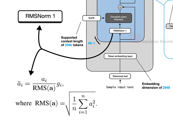
# RMSNorm function: scales the input tensor by the reciprocal of its root mean square
def rms_norm(tensor, norm_weights):
    input_dtype = tensor.dtype
    tensor_float = tensor.to(torch.float32)
    # Calculate the variance (mean of squares)
    variance = tensor_float.pow(2).mean(-1, keepdim=True)
    # Normalize by multiplying with the reciprocal square root of the variance
    normalized_tensor = tensor_float * torch.rsqrt(variance + norm_eps)
    # Apply the learnable weights and cast back to the original dtype
    return (normalized_tensor * norm_weights).to(input_dtype)

        我们将使用来自 layers_0 的注意力权重（attention weights）来对尚未归一化的嵌入向量进行归一化处理。之所以选用 layer_0，是因为我们当前正在构建 Qwen 3 架构的第一层。

# Apply RMSNorm to the embeddings using the weights 
# for the first layer's input
token_embeddings_normalized = rms_norm(
    token_embeddings_unnormalized, 
    model_weights["model.layers.0.input_layernorm.weight"]
)
print("Shape of the normalized token embeddings:", token_embeddings_normalized.shape)

#### OUTPUT ####
Shape of the normalized token embeddings: torch.Size([17, 1024])
#### OUTPUT ####

        经过归一化处理后，张量的形状保持不变，但其中的数值现已完成归一化，可以输入到注意力机制（attention mechanism）中使用了。

7 分组查询注意力机制（Grouped-Query Attention）

        接下来，我们将生成查询向量（Query，Q）、键向量（Key，K）和值向量（Value，V）。这些预训练得到的权重被存储在大型组合矩阵中。我们需要对这些矩阵进行重新调整形状（reshape），以分离出针对我们 16 个注意力头（attention heads）各自的权重。

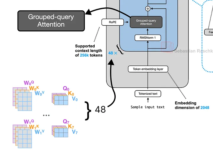
        该模型采用了一种名为分组查询注意力（Grouped-Query Attention，简称 GQA）的优化策略：在 16 个查询头（Query heads）中共享较少数量的键头（Key heads）和值头（Value heads）——具体为 8 个。这种设计能在几乎不损失模型性能的前提下，有效降低计算开销。

# Unpack the query weights into 16 heads
q_layer0 = model_weights["model.layers.0.self_attn.q_proj.weight"]
q_layer0 = q_layer0.view(n_heads, head_dim, dim)

# Unpack the key weights into 8 shared heads
k_layer0 = model_weights["model.layers.0.self_attn.k_proj.weight"]
k_layer0 = k_layer0.view(n_kv_heads, head_dim, dim)

# Unpack the value weights into 8 shared heads
v_layer0 = model_weights["model.layers.0.self_attn.v_proj.weight"]
v_layer0 = v_layer0.view(n_kv_heads, head_dim, dim)

        接下来，我们将通过将已归一化的嵌入向量（normalized embeddings）与当前注意力头的权重相乘，来计算第一个注意力头（head）对应的查询向量（Q）、键向量（K）和值向量（V）。

# Get the weights for the first head (head 0)
q_layer0_head0 = q_layer0[0]
k_layer0_head0 = k_layer0[0] # The first Q head uses the first KV head
v_layer0_head0 = v_layer0[0]

# Calculate the Q, K, and V vectors for each of the 17 tokens
q_per_token = torch.matmul(token_embeddings_normalized, q_layer0_head0.T)
k_per_token = torch.matmul(token_embeddings_normalized, k_layer0_head0.T)
v_per_token = torch.matmul(token_embeddings_normalized, v_layer0_head0.T)

# Verify the shape of the query vectors
print("Shape of Query vectors per token:", q_per_token.shape)


#### OUTPUT ####
Shape of Query vectors per token: torch.Size([17, 128])
#### OUTPUT ####

        目前，我们的 17 个词元（tokens）中的每一个，在第一个注意力头（head）中都分别拥有一个维度为 128 的查询向量（Q）、键向量（K）和值向量（V）。

8 旋转位置编码（Rotary Position Embedding）

        这些向量目前还不知道它们在序列中的位置信息。我们将使用 RoPE 通过对这些向量进行“旋转”操作，来注入位置信息。为了提高计算效率，我们可以预先计算出所有可能位置（直到最大序列长度为止）所对应的旋转角度。

# Pre-compute RoPE frequencies for all possible positions
max_seq_len = config["max_position_embeddings"]
freqs = 1.0 / (rope_theta ** (torch.arange(0, head_dim, 2) / head_dim))
t = torch.arange(max_seq_len)
freqs_for_each_token = torch.outer(t, freqs)
# `freqs_cis` is our lookup table of complex numbers for rotation
freqs_cis = torch.polar(torch.ones_like(freqs_for_each_token), freqs_for_each_token)

        freqs_cis 张量中存储的就是用于执行旋转操作的复数。我们可以针对单个词元（token）可视化这些旋转过程，从而观察每一对二维维度（2D pair of dimensions）是如何按照不同角度进行旋转的。

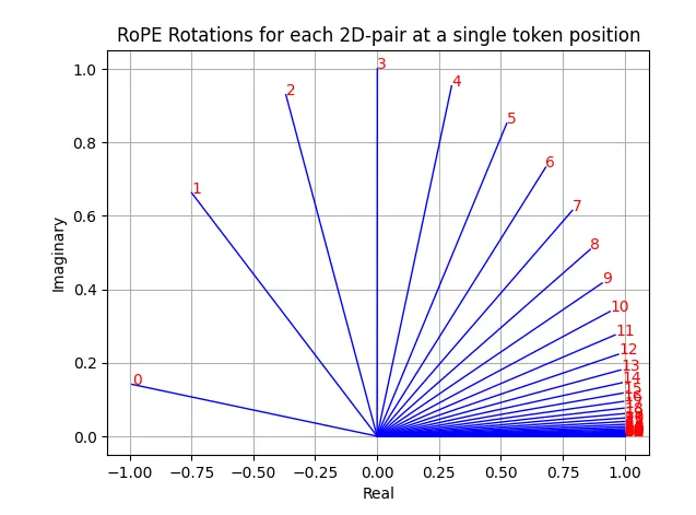
        我们将这些旋转操作应用到查询向量（Q）和键向量（K）上。具体而言，旋转是通过将向量视为复数，并执行逐元素乘法（element-wise multiplication）来完成的。

# Get the pre-computed rotations for our sequence of 17 tokens
freqs_cis_for_tokens = freqs_cis[:len(tokens)]

# --- Apply RoPE to Query vectors ---
# Reshape [17, 128] to [17, 64, 2] and view as complex numbers [17, 64]
q_per_token_as_complex_numbers = torch.view_as_complex(q_per_token.float().view(q_per_token.shape[0], -1, 2))
# Apply rotation via complex multiplication
q_per_token_rotated_complex = q_per_token_as_complex_numbers * freqs_cis_for_tokens
# Convert back to real numbers and reshape to [17, 128]
q_per_token_rotated = torch.view_as_real(q_per_token_rotated_complex).view(q_per_token.shape)

# --- Apply RoPE to Key vectors (same process) ---
k_per_token_as_complex_numbers = torch.view_as_complex(k_per_token.float().view(k_per_token.shape[0], -1, 2))
k_per_token_rotated_complex = k_per_token_as_complex_numbers * freqs_cis_for_tokens
k_per_token_rotated = torch.view_as_real(k_per_token_rotated_complex).view(k_per_token.shape)

print("Shape of rotated Query vectors:", q_per_token_rotated.shape)


#### OUTPUT ####
Shape of rotated Query vectors: torch.Size([17, 128])
#### OUTPUT ####

9 计算 Attention Scores

        现在，我们通过计算查询矩阵（query）和键矩阵（key）的点积（dot product）来求得注意力分数（attention scores）。这将生成一个形状为 [17, 17] 的矩阵，其中每个元素表示每个词元（token）应该“关注”（attend）其他每个词元的程度。为了稳定训练过程，我们会将这些分数除以头维度（head dimension）的平方根进行缩放（scale）。

# Calculate dot product of Q and K to get attention scores
qk_per_token = torch.matmul(q_per_token_rotated, k_per_token_rotated.T)
# Scale the scores for numerical stability
qk_per_token_scaled = qk_per_token / (head_dim**0.5)

        我们可以将这些原始注意力分数可视化为热力图（heatmap）。

# Calculate the raw attention scores by multiplying rotated Q and K vectors
qk_per_token = torch.matmul(q_per_token_rotated, k_per_token_rotated.T)

# Scale the attention scores by the square root of the head dimension
qk_per_token_scaled = qk_per_token / (head_dim**0.5)

# Visualize the raw attention scores before masking
def display_qk_heatmap(qk_matrix, title="Attention Heatmap"):
    _, ax = plt.subplots()
    im = ax.imshow(qk_matrix.to(torch.float32).detach(), cmap='viridis')
    ax.set_xticks(range(len(prompt_split_as_tokens)))
    ax.set_yticks(range(len(prompt_split_as_tokens)))
    ax.set_xticklabels(prompt_split_as_tokens, rotation=90)
    ax.set_yticklabels(prompt_split_as_tokens)
    ax.figure.colorbar(im, ax=ax)
    plt.title(title)
    plt.show()

display_qk_heatmap(qk_per_token_scaled, title="Raw Attention Scores (Before Masking)")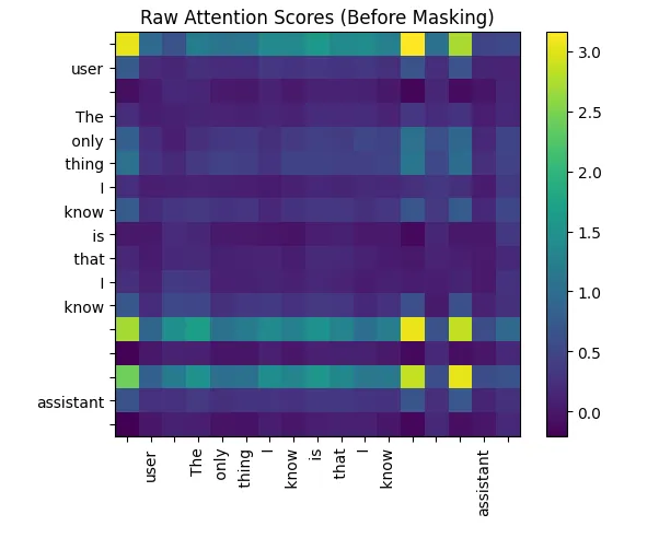

        为防止该自回归模型中的词元（tokens）“窥见”未来信息，我们会施加一个因果掩码（causal mask）。该掩码会将矩阵上三角区域内的所有注意力分数设为负无穷（negative infinity），这样经过 Softmax 函数处理后，这些位置的分数就会变为零。

# Create an upper-triangular mask with -inf values
mask = torch.full((len(tokens), len(tokens)), float("-inf"))
mask = torch.triu(mask, diagonal=1)

# Apply the mask to the scores
qk_per_token_masked = qk_per_token_scaled + mask

掩码矩阵像：

# Printing masking approach
print(mask)

#### OUTPUT ####
tensor([[0., -inf, -inf, -inf, -inf, -inf, -inf, -inf, -inf, -inf, -inf, -inf, -inf, -inf, -inf, -inf, -inf],
        [0., 0., -inf, -inf, -inf, -inf, -inf, -inf, -inf, -inf, -inf, -inf, -inf, -inf, -inf, -inf, -inf],
        [0., 0., 0., -inf, -inf, -inf, -inf, -inf, -inf, -inf, -inf, -inf, -inf, -inf, -inf, -inf, -inf],
        [0., 0., 0., 0., -inf, -inf, -inf, -inf, -inf, -inf, -inf, -inf, -inf, -inf, -inf, -inf, -inf],
        [0., 0., 0., 0., 0., -inf, -inf, -inf, -inf, -inf, -inf, -inf, -inf, -inf, -inf, -inf, -inf],
        [0., 0., 0., 0., 0., 0., -inf, -inf, -inf, -inf, -inf, -inf, -inf, -inf, -inf, -inf, -inf],
        [0., 0., 0., 0., 0., 0., 0., -inf, -inf, -inf, -inf, -inf, -inf, -inf, -inf, -inf, -inf],
        [0., 0., 0., 0., 0., 0., 0., 0., -inf, -inf, -inf, -inf, -inf, -inf, -inf, -inf, -inf],
        [0., 0., 0., 0., 0., 0., 0., 0., 0., -inf, -inf, -inf, -inf, -inf, -inf, -inf, -inf],
        [0., 0., 0., 0., 0., 0., 0., 0., 0., 0., -inf, -inf, -inf, -inf, -inf, -inf, -inf],
        [0., 0., 0., 0., 0., 0., 0., 0., 0., 0., 0., -inf, -inf, -inf, -inf, -inf, -inf],
        [0., 0., 0., 0., 0., 0., 0., 0., 0., 0., 0., 0., -inf, -inf, -inf, -inf, -inf],
        [0., 0., 0., 0., 0., 0., 0., 0., 0., 0., 0., 0., 0., -inf, -inf, -inf, -inf],
        [0., 0., 0., 0., 0., 0., 0., 0., 0., 0., 0., 0., 0., 0., -inf, -inf, -inf],
        [0., 0., 0., 0., 0., 0., 0., 0., 0., 0., 0., 0., 0., 0., 0., -inf, -inf],
        [0., 0., 0., 0., 0., 0., 0., 0., 0., 0., 0., 0., 0., 0., 0., 0., -inf],
        [0., 0., 0., 0., 0., 0., 0., 0., 0., 0., 0., 0., 0., 0., 0., 0., 0.]])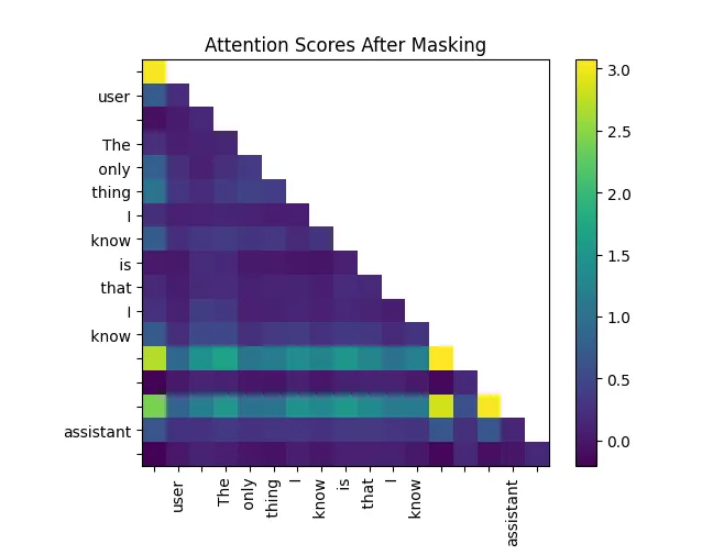

        最后，我们对这些分数（即注意力分数）施加 Softmax 函数，将其转换为概率分布（也就是注意力权重），并将其与值矩阵（Value matrix）相乘。这样便得到了值的加权求和结果，从而输出该注意力头（attention head）的最终结果。

# Apply softmax to turn scores into probabilities
qk_per_token_after_masking_after_softmax = torch.nn.functional.softmax(qk_per_token_masked.float(), dim=1).to(torch.bfloat16)
# Multiply the attention weights by the Value vectors
qkv_attention = torch.matmul(qk_per_token_after_masking_after_softmax, v_per_token)

print("Shape of the final attention output for Head 0:", qkv_attention.shape)


#### OUTPUT ####
Shape of the final attention output for Head 0: torch.Size([17, 128])
#### OUTPUT ####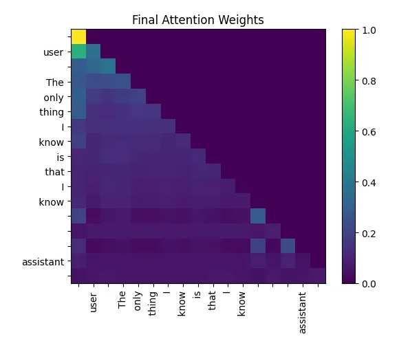

        该输出是一个新的 [17, 128] 张量，其中每个词元（token）的向量现在都包含了来自所有前面词元的上下文信息。

10 实现多头注意力机制（Multi-Head Attention）

        接下来，我们通过循环为全部 16 个注意力头（heads）重复上述自注意力（self-attention）过程。每个注意力头都会输出一个 [17, 128] 的张量，我们将这些输出收集到一个列表中。

（通过会将多个注意力头设置成新维度，这里主要方便读者阅读，采用循环操作）

# Create an empty list to store the attention output of each head.
qkv_attention_store = []

# Iterate over each of the 16 attention heads.
for head in range(n_heads):
    # Get the Q, K, and V weights for the current head.
    # Note the use of `head // 4` for K and V due to Grouped-Query Attention.
    # Every 4 query heads share the same key and value heads.
    q_layer0_head = q_layer0[head]
    k_layer0_head = k_layer0[head // (n_heads // n_kv_heads)]
    v_layer0_head = v_layer0[head // (n_heads // n_kv_heads)]

    # Project the normalized embeddings into Q, K, and V vectors for this head.
    q_per_token = torch.matmul(token_embeddings_normalized, q_layer0_head.T)
    k_per_token = torch.matmul(token_embeddings_normalized, k_layer0_head.T)
    v_per_token = torch.matmul(token_embeddings_normalized, v_layer0_head.T)

    # Apply RoPE to the Q and K vectors for this head.
    q_per_token_split_into_pairs = q_per_token.float().view(q_per_token.shape[0], -1, 2)
    q_per_token_as_complex_numbers = torch.view_as_complex(q_per_token_split_into_pairs)
    q_per_token_as_complex_numbers_rotated = q_per_token_as_complex_numbers * freqs_cis_for_tokens
    q_per_token_split_into_pairs_rotated = torch.view_as_real(q_per_token_as_complex_numbers_rotated)
    q_per_token_rotated = q_per_token_split_into_pairs_rotated.view(q_per_token.shape)

    k_per_token_split_into_pairs = k_per_token.float().view(k_per_token.shape[0], -1, 2)
    k_per_token_as_complex_numbers = torch.view_as_complex(k_per_token_split_into_pairs)
    k_per_token_as_complex_numbers_rotated = k_per_token_as_complex_numbers * freqs_cis_for_tokens
    k_per_token_split_into_pairs_rotated = torch.view_as_real(k_per_token_as_complex_numbers_rotated)
    k_per_token_rotated = k_per_token_split_into_pairs_rotated.view(k_per_token.shape)

    # Calculate and scale the attention scores.
    qk_per_token = torch.matmul(q_per_token_rotated, k_per_token_rotated.T) / (head_dim**0.5)

    # Apply the causal mask.
    qk_per_token_masked = qk_per_token + mask

    # Apply softmax to get the attention weights.
    qk_per_token_after_masking_after_softmax = torch.nn.functional.softmax(qk_per_token_masked.float(), dim=1).to(torch.bfloat16)

    # Aggregate the Value vectors using the attention weights.
    qkv_attention = torch.matmul(qk_per_token_after_masking_after_softmax, v_per_token)
    
    # Append the result of this head to our list.
    qkv_attention_store.append(qkv_attention)

        在循环结束后，我们将这 16 个注意力头的输出拼接（concatenate）成一个大的单一张量，其尺寸为 [17, 2048]（即 16 × 128 = 2048）。随后，我们使用输出权重矩阵 o_proj，将这个大张量投影（project）回模型原本的维度（1024），完成多头注意力机制的最终输出。

# Concatenate the outputs from all 16 heads along the last dimension
stacked_qkv_attention = torch.cat(qkv_attention_store, dim=-1)

# Get the output projection weights
w_layer0 = model_weights["model.layers.0.self_attn.o_proj.weight"]

# Project the concatenated outputs back to the model's hidden dimension
embedding_delta = torch.matmul(stacked_qkv_attention, w_layer0.T)

        最终得到的结果 embedding_delta 会被加回到该层的原始输入上。这就是第一个残差连接（residual connection）——这项关键技术能够通过让梯度更顺畅地流动，从而有效支持非常深层网络的训练。

# Add the output of the attention block back to its input (residual connection)
embedding_after_attention = token_embeddings_unnormalized + embedding_delta

11 混合专家模块（Mixture-of-Experts）

        这是 Transformer 块中的第二个子层。首先，我们会对该子层的输入施加预归一化（pre-normalization）操作。

# Apply RMSNorm before the MoE block, using the 'post_attention_layernorm' weights
embedding_after_attention_normalized = rms_norm(
    embedding_after_attention, 
    model_weights["model.layers.0.post_attention_layernorm.weight"]
)

        接下来，router（router，这里是一个简单的线性层）会计算分数，用于决定每个词元（token）应该被发送到两个专家（experts）中的哪一个。

# --- Step 1: The MoE Router ---
# The router is a simple linear layer that determines which expert to send each token to.
# It projects our [17, 1024] tensor to a [17, num_experts] tensor of scores (logits).
gate = model_weights["model.layers.0.mlp.gate.weight"]
router_logits = torch.matmul(embedding_after_attention_normalized, gate.T)

# We apply softmax to the logits to get probabilities, and then find the expert with the
# highest probability for each token.
routing_weights = torch.nn.functional.softmax(router_logits.float(), dim=1).to(torch.bfloat16)
routing_expert_indices = torch.argmax(routing_weights, dim=1)

print("Router logits shape:", router_logits.shape)
print("Expert chosen for each of the 17 tokens:", routing_expert_indices)

# --- Step 2: The Expert Layers ---
# Each expert is a SwiGLU-style Feed-Forward Network.
expert0_w1 = model_weights["model.layers.0.mlp.experts.0.gate_proj.weight"]
expert0_w2 = model_weights["model.layers.0.mlp.experts.0.down_proj.weight"]
expert0_w3 = model_weights["model.layers.0.mlp.experts.0.up_proj.weight"]

expert1_w1 = model_weights["model.layers.0.mlp.experts.1.gate_proj.weight"]
expert1_w2 = model_weights["model.layers.0.mlp.experts.1.down_proj.weight"]
expert1_w3 = model_weights["model.layers.0.mlp.experts.1.up_proj.weight"]

# --- Step 3: Process tokens with their chosen expert ---
final_expert_output = torch.zeros_like(embedding_after_attention_normalized)

#### OUTPUT ####
Router logits shape: torch.Size([17, 2])
Expert chosen for each of the 17 tokens: tensor([1, 1, 1, 1, 1, 1, 1, 1, 1, 1, 1, 1, 1, 1, 1, 1, 1])
#### OUTPUT ####

        在本例中，router 决定将全部 17 个词元（tokens）都路由至专家 1。接下来，我们会将每个词元的嵌入向量（embedding）送入其所选专家的前馈神经网络（Feed-Forward Network，简称 FFN）进行处理，然后将各专家的输出结果按照路由器给出的路由概率进行加权合并。

# Initialize a tensor to store the final output from the experts
final_expert_output = torch.zeros_like(embedding_after_attention_normalized)

# Loop through each token and process it with its chosen expert
for i, token_embedding in enumerate(embedding_after_attention_normalized):
    chosen_expert_index = routing_expert_indices[i]

    # (Get weights for the chosen expert and apply the FFN logic)
    # Get the weights for the chosen expert
    if chosen_expert_index == 0:
        w1, w2, w3 = expert0_w1, expert0_w2, expert0_w3
    else:
        w1, w2, w3 = expert1_w1, expert1_w2, expert1_w3
    
    # Apply the SwiGLU activation for this token's chosen expert
    silu_output = torch.nn.functional.silu(torch.matmul(token_embedding, w1.T))
    gated_output = silu_output * torch.matmul(token_embedding, w3.T)
    expert_output = torch.matmul(gated_output, w2.T)

    # Weight the expert's output by its routing probability
    final_expert_output[i] = expert_output * routing_weights[i, chosen_expert_index]

        最后，我们将混合专家模块（MoE Block）的输出结果，与注意力模块（attention block）的输出相加。这是第二个残差连接（residual connection），至此，整个 Transformer 层的构建便完成了。

# Second residual connection: add the output of the MoE block to its input
layer_0_embedding = embedding_after_attention + final_expert_output

12 整合所有模块

        现在我们已经集齐了所有组件，可以通过循环遍历全部 28 层来构建完整的模型。前一层的输出将作为下一层的输入。

# The final embedding starts as the output from the token embedding layer.
# We will update this tensor in-place as it passes through the layers.
final_embedding = token_embeddings_unnormalized

# Loop through each of the 28 layers of the transformer.
for layer in range(n_layers):
    
    # --- Attention Sub-Layer ---
    
    # 1. RMS Normalization before attention
    attention_input = rms_norm(final_embedding, model_weights[f"model.layers.{layer}.input_layernorm.weight"])
    
    # 2. Multi-Head Attention
    q_layer = model_weights[f"model.layers.{layer}.self_attn.q_proj.weight"].view(n_heads, head_dim, dim)
    k_layer = model_weights[f"model.layers.{layer}.self_attn.k_proj.weight"].view(n_kv_heads, head_dim, dim)
    v_layer = model_weights[f"model.layers.{layer}.self_attn.v_proj.weight"].view(n_kv_heads, head_dim, dim)
    w_layer = model_weights[f"model.layers.{layer}.self_attn.o_proj.weight"]
    
    qkv_attention_store = []
    for head in range(n_heads):
        q_layer_head = q_layer[head]
        k_layer_head = k_layer[head // (n_heads // n_kv_heads)]
        v_layer_head = v_layer[head // (n_heads // n_kv_heads)]

        q_per_token = torch.matmul(attention_input, q_layer_head.T)
        k_per_token = torch.matmul(attention_input, k_layer_head.T)
        v_per_token = torch.matmul(attention_input, v_layer_head.T)

        q_per_token_rotated = torch.view_as_real(torch.view_as_complex(q_per_token.float().view(q_per_token.shape[0], -1, 2)) * freqs_cis_for_tokens).view(q_per_token.shape)
        k_per_token_rotated = torch.view_as_real(torch.view_as_complex(k_per_token.float().view(k_per_token.shape[0], -1, 2)) * freqs_cis_for_tokens).view(k_per_token.shape)
        
        qk_per_token = torch.matmul(q_per_token_rotated, k_per_token_rotated.T) / (head_dim**0.5)
        qk_per_token_masked = qk_per_token + mask
        qk_per_token_after_masking_after_softmax = torch.nn.functional.softmax(qk_per_token_masked.float(), dim=1).to(torch.bfloat16)
        
        qkv_attention = torch.matmul(qk_per_token_after_masking_after_softmax, v_per_token)
        qkv_attention_store.append(qkv_attention)
        
    stacked_qkv_attention = torch.cat(qkv_attention_store, dim=-1)
    embedding_delta = torch.matmul(stacked_qkv_attention, w_layer.T)
    
    # 3. First Residual Connection
    embedding_after_attention = final_embedding + embedding_delta
    
    # --- Mixture-of-Experts Sub-Layer ---
    
    # 1. RMS Normalization before MoE
    moe_input = rms_norm(embedding_after_attention, model_weights[f"model.layers.{layer}.post_attention_layernorm.weight"])
    
    # 2. Router
    gate = model_weights[f"model.layers.{layer}.mlp.gate.weight"]
    router_logits = torch.matmul(moe_input, gate.T)
    routing_weights = torch.nn.functional.softmax(router_logits.float(), dim=1).to(torch.bfloat16)
    routing_expert_indices = torch.argmax(routing_weights, dim=1)
    
    # 3. Expert Layers
    final_expert_output = torch.zeros_like(moe_input)
    
    expert0_w1 = model_weights[f"model.layers.{layer}.mlp.experts.0.gate_proj.weight"]
    expert0_w2 = model_weights[f"model.layers.{layer}.mlp.experts.0.down_proj.weight"]
    expert0_w3 = model_weights[f"model.layers.{layer}.mlp.experts.0.up_proj.weight"]

    expert1_w1 = model_weights[f"model.layers.{layer}.mlp.experts.1.gate_proj.weight"]
    expert1_w2 = model_weights[f"model.layers.{layer}.mlp.experts.1.down_proj.weight"]
    expert1_w3 = model_weights[f"model.layers.{layer}.mlp.experts.1.up_proj.weight"]
    
    for i, token_embedding in enumerate(moe_input):
        chosen_expert_index = routing_expert_indices[i]
        
        if chosen_expert_index == 0:
            w1, w2, w3 = expert0_w1, expert0_w2, expert0_w3
        else:
            w1, w2, w3 = expert1_w1, expert1_w2, expert1_w3
        
        silu_output = torch.nn.functional.silu(torch.matmul(token_embedding, w1.T))
        gated_output = silu_output * torch.matmul(token_embedding, w3.T)
        expert_output = torch.matmul(gated_output, w2.T)
        
        final_expert_output[i] = expert_output * routing_weights[i, chosen_expert_index]
        
    # 4. Second Residual Connection
    final_embedding = embedding_after_attention + final_expert_output

# --- Verify the final shape ---
print("Shape of the final embeddings after all layers:", final_embedding.shape)
#### OUTPUT ####
Shape of the final embeddings after all layers: torch.Size([17, 1024])
#### OUTPUT ####

13 生成最终输出

        现在，我们得到了最终的嵌入向量（embedding），它代表了模型对于下一个词元（token）的预测结果。该张量的形状为 [17, 1024]。首先，我们会对其施加最后一次 RMSNorm 归一化操作。

# Apply the final layer normalization
final_embedding_normalized = rms_norm(final_embedding, model_weights["model.norm.weight"])

        要获得最终的预测结果，我们只需要取序列中最后一个词元（token）对应的嵌入向量（embedding）。这是一个维度为 [1024] 的向量。接着，我们将这个向量与语言模型头部权重（language model head weights，该权重通常与词元嵌入层的权重共享/tied）相乘，从而得到词汇表中每个词对应的得分，也称为 logits（未归一化的预测分数）。

# The LM Head weights are the same as the embedding weights (weight tying)
lm_head_weights = model_weights["model.embed_tokens.weight"]

# We only care about the last token's output to predict the next token
last_token_embedding = final_embedding_normalized[-1]

# Calculate the logits by multiplying with the LM Head
logits = torch.matmul(last_token_embedding, lm_head_weights.T)

print("Shape of the final logits:", logits.shape)

#### OUTPUT ####
Shape of the final logits: torch.Size([151936])
#### OUTPUT ####

        具有最高 logits 分数的词元即为我们模型的预测结果。我们使用 argmax 函数来找出该词元在词汇表中的索引。

# Find the token ID with the highest score
next_token_id = torch.argmax(logits, dim=-1)
print(f"Predicted Token ID: {next_token_id.item()}")

# Decode the ID back to a string to see the predicted word
predicted_word = tokenizer.decode([next_token_id.item()])
print(f"\nPredicted Word: '{predicted_word}'")


#### OUTPUT ####
Predicted Token ID: 12454
Predicted Word: 'nothing'
#### OUTPUT ####

        因此，在输入提示词 ...assistant\n，模型预测下一个最可能的词是“nothing”。这虽然只是一个单词元（单 token）的生成示例，但它充分证明：我们从头开始实现的整个 Qwen 3 混合专家（MoE）架构运行正确、功能完备。您只需修改开头的 prompt 变量，并相应调整词元张量（token tensor）的构建方式，就可以尝试使用不同的输入文本进行实验。