《从零构建大模型》系列(19):实现带可训练权重的自注意力机制——大语言模型的核心引擎
本文详细解析了可训练自注意力机制的实现原理与应用。文章首先解释了可训练权重的重要性,包括增强模型适应性和表达能力等核心优势。随后分步演示了自注意力机制的完整实现过程:从初始化权重矩阵、计算QKV向量,到注意力分数计算、缩放归一化,最终生成上下文向量。文中对比了两种实现方式(基础参数实现与优化线性层实现),并深入探讨了缩放点积注意力的数学原理。此外,文章还分析了自注意力在GPT等大模型中的实际应用配

目录
可训练权重赋予模型学习能力:本节将深入实现带有可训练权重的自注意力机制,这是Transformer架构的核心创新,也是GPT等大语言模型成功的关键所在。
一、可训练自注意力机制详解
1.1 为什么需要可训练权重?
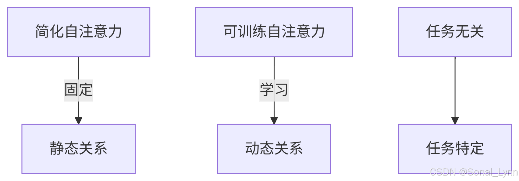
核心优势:
-
适应性:模型可以学习特定任务的最佳表示
-
表达能力:增强捕捉复杂模式的能力
-
泛化能力:在不同上下文和任务中表现更好
1.2 查询(Q)、键(K)、值(V)三元组
其中:
-
X:输入嵌入矩阵
-
:可训练权重矩阵
二、逐步实现可训练自注意力
2.1 初始化权重矩阵
import torch
import torch.nn as nn

# 输入输出维度设置
d_in = 3  # 输入维度
d_out = 2  # 输出维度

# 初始化可训练权重矩阵
torch.manual_seed(123)
W_query = nn.Parameter(torch.rand(d_in, d_out), requires_grad=True)
W_key = nn.Parameter(torch.rand(d_in, d_out), requires_grad=True)
W_value = nn.Parameter(torch.rand(d_in, d_out), requires_grad=True)

print("W_query:\n", W_query)
print("W_key:\n", W_key)
print("W_value:\n", W_value)
2.2 计算查询、键、值向量
# 输入数据
inputs = torch.tensor([
    [0.43, 0.15, 0.89],  # Your
    [0.57, 0.85, 0.64],  # journey
    [0.55, 0.87, 0.66],  # starts
    [0.77, 0.25, 0.10],  # with
    [0.05, 0.80, 0.55],  # one
    [0.48, 0.69, 0.35]   # step
])

# 计算查询向量(以"journey"为例)
x_2 = inputs[1]  # 第二个词元"journey"
query_2 = x_2 @ W_query
print("\n查询向量(query_2):", query_2)

# 计算所有键和值向量
keys = inputs @ W_key
values = inputs @ W_value
print("\n键向量(keys):\n", keys)
print("\n值向量(values):\n", values)
2.3 计算注意力分数
# 计算"journey"与其他所有词的注意力分数
attn_scores_2 = query_2 @ keys.T
print("\n注意力分数:", attn_scores_2)
2.4 缩放与Softmax归一化
# 缩放因子:键向量维度的平方根
d_k = keys.shape[-1]
scaled_attn_scores = attn_scores_2 / (d_k ** 0.5)

# Softmax归一化
attn_weights_2 = torch.softmax(scaled_attn_scores, dim=-1)
print("\n注意力权重:", attn_weights_2)
print("权重和:", attn_weights_2.sum().item())  # 应为1.0
2.5 计算上下文向量
# 加权求和值向量
context_vec_2 = attn_weights_2 @ values
print("\n上下文向量:", context_vec_2)
三、完整自注意力类实现
3.1 基础实现(使用nn.Parameter)
class SelfAttention_v1(nn.Module):
    def __init__(self, d_in, d_out):
        super().__init__()
        # 初始化可训练权重
        self.W_query = nn.Parameter(torch.rand(d_in, d_out))
        self.W_key = nn.Parameter(torch.rand(d_in, d_out))
        self.W_value = nn.Parameter(torch.rand(d_in, d_out))

    def forward(self, x):
        # 计算Q, K, V
        queries = x @ self.W_query
        keys = x @ self.W_key
        values = x @ self.W_value

        # 计算注意力分数
        attn_scores = queries @ keys.T

        # 缩放
        d_k = keys.shape[-1]
        scaled_attn_scores = attn_scores / (d_k ** 0.5)

        # Softmax归一化
        attn_weights = torch.softmax(scaled_attn_scores, dim=-1)

        # 计算上下文向量
        context_vec = attn_weights @ values

        return context_vec

# 测试
torch.manual_seed(123)
sa_v1 = SelfAttention_v1(d_in, d_out)
output = sa_v1(inputs)
print("\nSelfAttention_v1输出:\n", output)
3.2 优化实现(使用nn.Linear)
class SelfAttention_v2(nn.Module):
    def __init__(self, d_in, d_out, qkv_bias=False):
        super().__init__()
        # 使用nn.Linear代替手动权重管理
        self.W_query = nn.Linear(d_in, d_out, bias=qkv_bias)
        self.W_key = nn.Linear(d_in, d_out, bias=qkv_bias)
        self.W_value = nn.Linear(d_in, d_out, bias=qkv_bias)

        # 更稳定的初始化
        self._init_weights()

    def _init_weights(self):
        # Xavier/Glorot初始化
        nn.init.xavier_uniform_(self.W_query.weight)
        nn.init.xavier_uniform_(self.W_key.weight)
        nn.init.xavier_uniform_(self.W_value.weight)

        if self.W_query.bias is not None:
            nn.init.zeros_(self.W_query.bias)
            nn.init.zeros_(self.W_key.bias)
            nn.init.zeros_(self.W_value.bias)

    def forward(self, x):
        # 计算Q, K, V
        queries = self.W_query(x)
        keys = self.W_key(x)
        values = self.W_value(x)

        # 计算注意力分数
        attn_scores = queries @ keys.transpose(-2, -1)

        # 缩放
        d_k = keys.size(-1)
        scaled_attn_scores = attn_scores / (d_k ** 0.5)

        # Softmax归一化
        attn_weights = torch.softmax(scaled_attn_scores, dim=-1)

        # 计算上下文向量
        context_vec = attn_weights @ values

        return context_vec

# 测试
torch.manual_seed(123)
sa_v2 = SelfAttention_v2(d_in, d_out)
output = sa_v2(inputs)
print("\nSelfAttention_v2输出:\n", output)
3.3 两种实现方式对比
| 特性 | SelfAttention_v1 | SelfAttention_v2 |
|---|---|---|
| 权重管理 | 手动管理 | 自动管理 |
| 初始化 | 简单随机 | 优化初始化 |
| 偏置支持 | 无 | 可选 |
| 代码简洁性 | 较低 | 较高 |
| 可扩展性 | 有限 | 良好 |
| 实际应用 | 教学演示 | 生产环境 |
四、缩放点积注意力的数学原理
4.1 缩放因子的必要性
为什么需要 ?
-
当 $d_k$ 较大时,点积结果可能非常大
-
导致 softmax 进入梯度饱和区
-
梯度变小,训练困难
# 缩放效果演示
d_k_large = 1024
unscaled = torch.randn(1, d_k_large) @ torch.randn(d_k_large, 1)
scaled = unscaled / (d_k_large ** 0.5)

print(f"未缩放: {unscaled.item():.2f}, 缩放后: {scaled.item():.2f}")
# 示例输出: 未缩放: 32.15, 缩放后: 1.00
4.2 注意力机制的可视化
import matplotlib.pyplot as plt
import seaborn as sns

def visualize_attention(model, inputs):
    # 获取注意力权重
    with torch.no_grad():
        queries = model.W_query(inputs)
        keys = model.W_key(inputs)
        attn_scores = queries @ keys.T
        d_k = keys.shape[-1]
        scaled_attn_scores = attn_scores / (d_k ** 0.5)
        attn_weights = torch.softmax(scaled_attn_scores, dim=-1)

    # 可视化
    plt.figure(figsize=(10, 8))
    sns.heatmap(attn_weights.numpy(),
                annot=True, fmt=".2f",
                xticklabels=["Your", "journey", "starts", "with", "one", "step"],
                yticklabels=["Your", "journey", "starts", "with", "one", "step"])
    plt.title("可训练自注意力权重")
    plt.xlabel("Key")
    plt.ylabel("Query")
    plt.show()

# 可视化
visualize_attention(sa_v1, inputs)
五、在大语言模型中的实际应用
5.1 GPT中的自注意力层
class GPTAttentionBlock(nn.Module):
    def __init__(self, d_model, n_heads):
        super().__init__()
        self.d_model = d_model
        self.n_heads = n_heads
        self.head_dim = d_model // n_heads

        # 查询、键、值投影
        self.W_q = nn.Linear(d_model, d_model)
        self.W_k = nn.Linear(d_model, d_model)
        self.W_v = nn.Linear(d_model, d_model)

        # 输出投影
        self.W_o = nn.Linear(d_model, d_model)

    def forward(self, x):
        batch_size, seq_len, _ = x.shape

        # 线性投影
        Q = self.W_q(x)
        K = self.W_k(x)
        V = self.W_v(x)

        # 分割多头
        Q = Q.view(batch_size, seq_len, self.n_heads, self.head_dim).transpose(1, 2)
        K = K.view(batch_size, seq_len, self.n_heads, self.head_dim).transpose(1, 2)
        V = V.view(batch_size, seq_len, self.n_heads, self.head_dim).transpose(1, 2)

        # 计算注意力分数
        attn_scores = Q @ K.transpose(-2, -1) / (self.head_dim ** 0.5)

        # 应用softmax
        attn_weights = torch.softmax(attn_scores, dim=-1)

        # 加权求和
        context = attn_weights @ V

        # 合并多头
        context = context.transpose(1, 2).contiguous()
        context = context.view(batch_size, seq_len, self.d_model)

        # 输出投影
        output = self.W_o(context)

        return output
5.2 实际模型配置对比
| 模型 | 隐藏维度 | 注意力头数 | 头维度 | 总参数量 |
|---|---|---|---|---|
| GPT-2 Small | 768 | 12 | 64 | 117M |
| GPT-2 Medium | 1024 | 16 | 64 | 345M |
| GPT-2 Large | 1280 | 20 | 64 | 774M |
| GPT-3 175B | 12288 | 96 | 128 | 175B |
六、训练过程中的行为分析
6.1 权重演变可视化
def track_attention_evolution(model, inputs, word_idx, num_epochs=100):
optimizer = torch.optim.Adam(model.parameters(), lr=0.01)
context_vecs = []
# 简单训练任务:使输出接近某种目标
target = torch.randn(d_out)
for epoch in range(num_epochs):
optimizer.zero_grad()
output = model(inputs)
loss = torch.nn.functional.mse_loss(output[word_idx], target)
loss.backward()
optimizer.step()
# 记录上下文向量
context_vecs.append(output[word_idx].detach().numpy())
# 可视化演变
plt.figure(figsize=(12, 6))
context_vecs = np.array(context_vecs)
for i in range(d_out):
plt.plot(context_vecs[:, i], label=f'维度 {i+1}')
plt.title(f"词元 '{['Your','journey','starts','with','one','step'][word_idx]}' 的上下文向量演变")
plt.xlabel("训练周期")
plt.ylabel("值")
plt.legend()
plt.grid(True)
plt.show()
# 跟踪"journey"的上下文向量演变
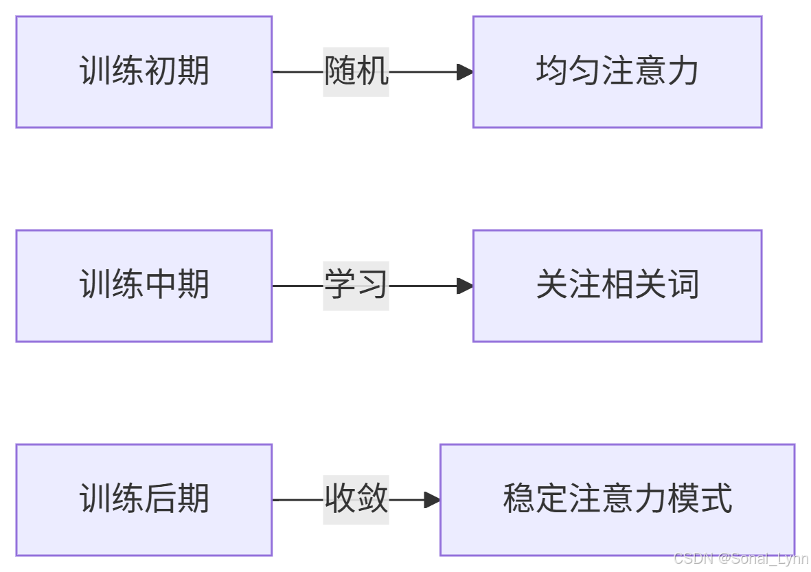
track_attention_evolution(sa_v1, inputs, word_idx=1)6.2 学习到的注意力模式变化
七、常见问题与解决方案
7.1 梯度消失/爆炸问题
解决方案:
-
权重初始化(如Xavier初始化)
-
梯度裁剪
-
Layer Normalization
class StableSelfAttention(nn.Module):
    def __init__(self, d_in, d_out):
        super().__init__()
        self.attn = SelfAttention_v2(d_in, d_out)
        self.norm = nn.LayerNorm(d_out)  # 添加层归一化

    def forward(self, x):
        residual = x
        x = self.attn(x)
        return self.norm(x + residual)  # 残差连接
7.2 计算效率优化
def efficient_attention(Q, K, V):
    # 分块计算,减少内存占用
    batch_size, seq_len, _ = Q.shape
    chunk_size = 64  # 根据GPU内存调整

    output = torch.zeros_like(V)
    for i in range(0, seq_len, chunk_size):
        Q_chunk = Q[:, i:i+chunk_size]
        attn_scores = Q_chunk @ K.transpose(-2, -1)
        attn_weights = torch.softmax(attn_scores / (K.shape[-1]**0.5), dim=-1)
        output[:, i:i+chunk_size] = attn_weights @ V

    return output
八、高级话题:查询、键、值的本质
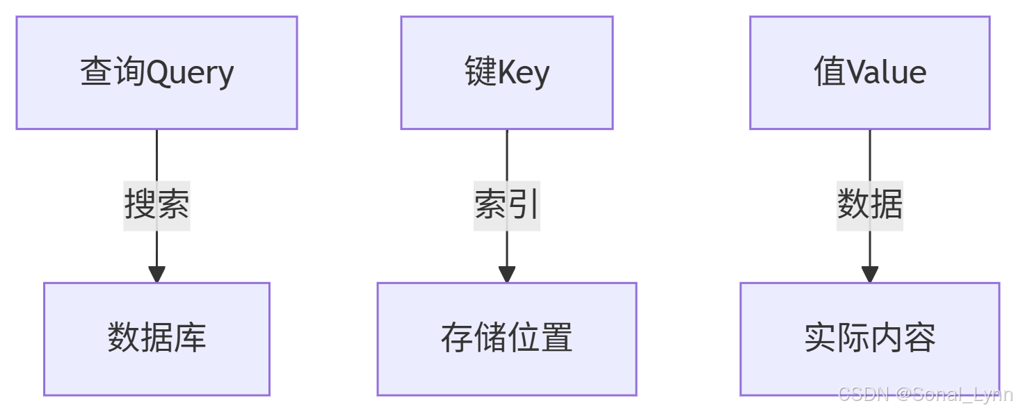
8.1 信息检索的类比
在注意力机制中:
-
查询:当前关注的词元("我想了解什么?")
-
键:所有词元的标识("我能提供什么信息?")
-
值:词元包含的实际内容("我的具体内容是什么?")
8.2 不同模型中的QKV实现
| 模型 | QKV处理 | 特点 |
|---|---|---|
| Transformer | 独立投影 | 标准实现 |
| GPT | 共享输入 | 自回归特性 |
| BERT | 双向融合 | 上下文双向关注 |
| T5 | 相对位置 | 位置感知注意力 |
九、总结与展望
9.1 关键收获
-
可训练权重:赋予模型学习不同表示空间的能力
-
缩放点积:解决大维度下的梯度消失问题
-
模块化实现:为构建更复杂架构奠定基础
9.2 下一步方向
-
因果注意力:添加掩码实现自回归生成
-
多头注意力:并行捕捉多种关系模式
-
性能优化:FlashAttention等加速技术
"可训练的自注意力机制是现代大语言模型的基础,它使模型能够动态地关注输入的不同部分,这是实现真正语境理解的关键突破。"

火山引擎开发者社区是火山引擎打造的AI技术生态平台,聚焦Agent与大模型开发,提供豆包系列模型(图像/视频/视觉)、智能分析与会话工具,并配套评测集、动手实验室及行业案例库。社区通过技术沙龙、挑战赛等活动促进开发者成长,新用户可领50万Tokens权益,助力构建智能应用。
更多推荐
 19
19 0
0- 0


 已为社区贡献9条内容

所有评论(0)