前言

本篇博客主要神经网络中最简单的网络模型，即单层感知机（Single Layer Perceptron），并基于pytorch框架实现该网络的搭建。虽然如今看来，该模型只能解决线性可分的问题，但作为神经网络的开山之作，仍值得学习。

1.单层感知机

1.1模型介绍

单层感知机网络结构可表示为下图所示（最近发现豆包的画图功能有进步，所以直接用豆包的图片了）：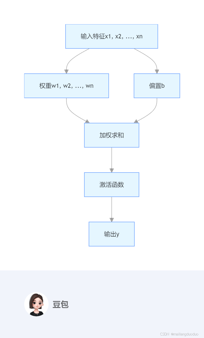

根据图示结构，得到的加权和可表示为：$$z=\sum _{i=1}^n{w}_i{x}_i+b=w^{T}x+b$$
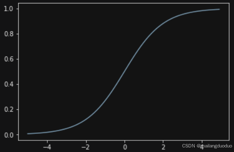
激活层一般选用Sigmoid 函数将输出值压缩到 0 到 1 之间，输出值大于 0.5 时，将其预测为正类；小于 0.5 时，预测为负类。

Sigmoid 函数如下：
$$\sigma (z)=\frac{1}{1+e^{-z}}$$
可视化结果为：

详细的模型介绍可参考：机器学习——感知机模型

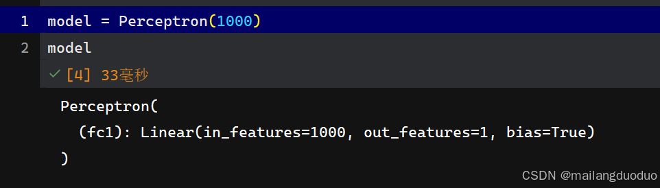
1.2模型搭建

这里使用pytorch框架搭建，直接定义一个线性层即可，具体代码如下：

class Perceptron(nn.Module):
    def __init__(self, input_dim):
        super(Perceptron, self).__init__()
        self.fc1 = nn.Linear(input_dim, 1)

    def forward(self, x_in):
        return torch.sigmoid(self.fc1(x_in))

2.数据集

2.1数据集介绍

这里的数据集是自制的，确定两个类别的中心点，围绕该中心点生成正态分布的坐标。

2.2代码介绍

LEFT_CENTER = (3, 3)
RIGHT_CENTER = (3, -2)
def get_toy_data(batch_size, left_center=LEFT_CENTER, right_center=RIGHT_CENTER):
    x_data = []
    y_targets = np.zeros(batch_size)
    for batch_i in range(batch_size):
        if np.random.random() > 0.5:
            x_data.append(np.random.normal(loc=left_center))
        else:
            x_data.append(np.random.normal(loc=right_center))
            y_targets[batch_i] = 1
    return torch.tensor(x_data, dtype=torch.float32), torch.tensor(y_targets, dtype=torch.float32)

这里的定义了一个函数，用来生产一个批量的数据及标签，因为使用的是随机数和0.5比大小，所以生成的两个类别数量基本一致，不会出现类不平衡现象。

2.3可视化

这里将随机生成的一个批量的数据进行可视化，代码如下：

X, y = get_toy_data(100)
# 可视化数据分布
plt.scatter(X[:,0], X[:,1], c=y)
plt.show()

运行结果：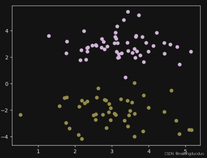

3.训练过程可视化

首先根据感知机模型的输出，将预测值大于0.5的置为1，小于0.5的值为零。同时将数据类型由tensor转换为np.int32类型

    y_pred = perceptron(x_data)
    y_pred = (y_pred > 0.5).long().data.numpy().astype(np.int32)

    x_data = x_data.data.numpy()
    y_truth = y_truth.data.numpy().astype(np.int32)

接着创建了两个嵌套列表，all_x和all_colors:

• all_x列表用来存储真实标签的情况，即真实标记为0的存储在all_x[0]列表中，真实标记为1的存储在all_x[1]列表中。
• all_colors列表用来存储对应标签的预测情况，如果预测正确就计为白色，错误计为黑色，和all_x列表内的元素一一对应，最后np.stack将其转换为numpy数组。

    n_classes = 2
    all_x = [[] for _ in range(n_classes)]
    all_colors = [[] for _ in range(n_classes)]
    
    colors = ['black', 'white']
    markers = ['o', '*']
    
    for x_i, y_pred_i, y_true_i in zip(x_data, y_pred, y_truth):
        all_x[y_true_i].append(x_i)
        if y_pred_i == y_true_i:
            all_colors[y_true_i].append("white")
        else:
            all_colors[y_true_i].append("black")
        #all_colors[y_true_i].append(colors[y_pred_i])

    all_x = [np.stack(x_list) for x_list in all_x]

接着将其进行可视化，类别0用mark[0]表示，类别1用mark[1]表示，预测正确颜色标记为白色，错误标记成黑色。

    if ax is None:
        _, ax = plt.subplots(1, 1, figsize=(10,10))
        
    for x_list, color_list, marker in zip(all_x, all_colors, markers):
        ax.scatter(x_list[:, 0], x_list[:, 1], edgecolor="black", marker=marker, facecolor=color_list, s=300)

此时已经完成预测结果的可视化，为了更好地观察结果，此处将分类的超平面也进行可视化输出，详细过程如下：
首先，确定横纵坐标的表示范围，直接使用所有坐标的最大值和最小值表示即可

    xlim = (min([x_list[:,0].min() for x_list in all_x]), 
            max([x_list[:,0].max() for x_list in all_x]))
            
    ylim = (min([x_list[:,1].min() for x_list in all_x]), 
            max([x_list[:,1].max() for x_list in all_x]))

这里定义一个网格，得到网格中每个点的坐标xy最终类型大小为（900,2）（此处是这个）

    xx = np.linspace(xlim[0], xlim[1], 30)
    yy = np.linspace(ylim[0], ylim[1], 30)
    YY, XX = np.meshgrid(yy, xx)
    xy = np.vstack([XX.ravel(), YY.ravel()]).T

接着将得到的xy坐标作为输入到感知机模型，得到对应的输出，输出的形状为(900,1)再将其调整为（30，30）

    Z = perceptron(torch.tensor(xy, dtype=torch.float32)).detach().numpy().reshape(XX.shape)

最后使用contour()绘制等高线即可，并添加上标题信息等内容：

    ax.contour(XX, YY, Z, colors='k', levels=levels, linestyles=linestyles)    
    
    plt.suptitle(title)
    
    if epoch is not None:
        plt.text(xlim[0], ylim[1], "Epoch = {}".format(str(epoch)))```

这里将上述过程封装成了一个函数，具体如下：

def visualize_results(perceptron, x_data, y_truth, n_samples=1000, ax=None, epoch=None,
                      title='', levels=[0.3, 0.4, 0.5], linestyles=['--', '-', '--']):
    y_pred = perceptron(x_data)
    y_pred = (y_pred > 0.5).long().data.numpy().astype(np.int32)

    x_data = x_data.data.numpy()
    y_truth = y_truth.data.numpy().astype(np.int32)

    n_classes = 2

    all_x = [[] for _ in range(n_classes)]
    all_colors = [[] for _ in range(n_classes)]
    
    colors = ['black', 'white']
    markers = ['o', '*']
    
    for x_i, y_pred_i, y_true_i in zip(x_data, y_pred, y_truth):
        all_x[y_true_i].append(x_i)
        if y_pred_i == y_true_i:
            all_colors[y_true_i].append("white")
        else:
            all_colors[y_true_i].append("black")
        #all_colors[y_true_i].append(colors[y_pred_i])

    all_x = [np.stack(x_list) for x_list in all_x]

    if ax is None:
        _, ax = plt.subplots(1, 1, figsize=(10,10))
        
    for x_list, color_list, marker in zip(all_x, all_colors, markers):
        ax.scatter(x_list[:, 0], x_list[:, 1], edgecolor="black", marker=marker, facecolor=color_list, s=300)
    
        
    xlim = (min([x_list[:,0].min() for x_list in all_x]), 
            max([x_list[:,0].max() for x_list in all_x]))
            
    ylim = (min([x_list[:,1].min() for x_list in all_x]), 
            max([x_list[:,1].max() for x_list in all_x]))
            
    # hyperplane
    
    xx = np.linspace(xlim[0], xlim[1], 30)
    yy = np.linspace(ylim[0], ylim[1], 30)
    YY, XX = np.meshgrid(yy, xx)
    xy = np.vstack([XX.ravel(), YY.ravel()]).T
    
    Z = perceptron(torch.tensor(xy, dtype=torch.float32)).detach().numpy().reshape(XX.shape)
    ax.contour(XX, YY, Z, colors='k', levels=levels, linestyles=linestyles)    
    
    plt.suptitle(title)
    
    if epoch is not None:
        plt.text(xlim[0], ylim[1], "Epoch = {}".format(str(epoch)))

接着就是训练过程了。

4.训练阶段

4.1超参数选择

首先定义一些超参数，包括学习率、输入尺寸、批量大小、一轮共有多少个批量，共有多少轮数。同时设置了随机种子，使得结果能够保持可复现。

lr = 0.01
input_dim = 2

batch_size = 1000
n_epochs = 12
n_batches = 5

seed = 1337

torch.manual_seed(seed)
torch.cuda.manual_seed_all(seed)
np.random.seed(seed)

4.2优化器与损失

这里选择的优化器为Adam，损失为二元交叉熵损失。

perceptron = Perceptron(input_dim=input_dim)
optimizer = optim.Adam(params=perceptron.parameters(), lr=lr)
bce_loss = nn.BCELoss()

4.3数据集加载

这里的数据集获取加载在每个批次里面，因此并没有完整的数据集，但为了可视化方便，选用第一次选取的批次作为可视化，代码如下：

x_data_static, y_truth_static = get_toy_data(batch_size)
fig, ax = plt.subplots(1, 1, figsize=(10,5))
visualize_results(perceptron, x_data_static, y_truth_static, ax=ax, title='Initial Model State')
plt.axis('off')
plt.show()

结果如下：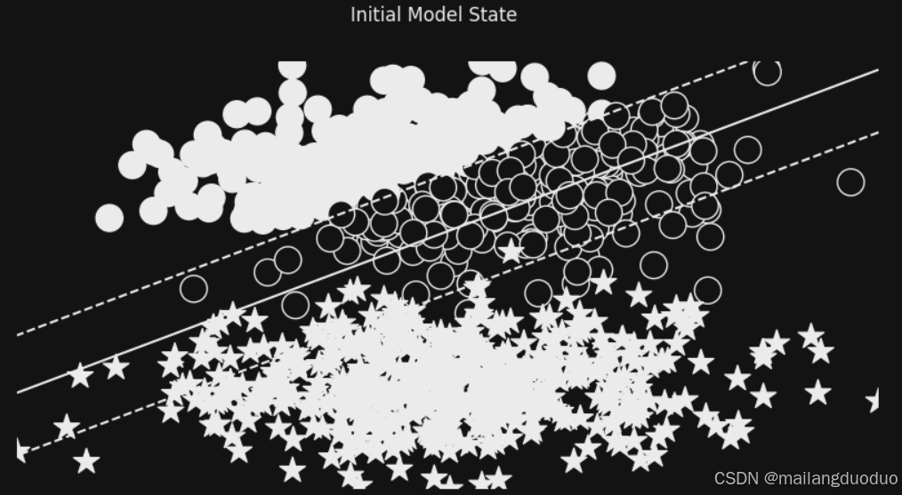

4.4训练过程

这里的训练过程并不是简单的，但epoch达到最大的epochs结束，而是增加了求他条件，损失需要小于0.3且连续两次的损失变化需要小于epsilon且epoch达到最大的epochs结束。这里选择的批量足够大，因此避免了损失的波动

losses = []
change = 1.0
last = 10.0
epsilon = 1e-3
epoch = 0
while change > epsilon or epoch < n_epochs or last > 0.3:
    for _ in range(n_batches):

        optimizer.zero_grad()
        x_data, y_target = get_toy_data(batch_size)
        y_pred = perceptron(x_data).squeeze()
        loss = bce_loss(y_pred, y_target)
        loss.backward()
        optimizer.step()
        
        
        loss_value = loss.item()
        losses.append(loss_value)

        change = abs(last - loss_value)
        last = loss_value
               
    fig, ax = plt.subplots(1, 1, figsize=(10,5))
    visualize_results(perceptron, x_data_static, y_truth_static, ax=ax, epoch=epoch, 
                      title=f"{loss_value}; {change}")
    plt.axis('off')
    epoch += 1
plt.show()

运行结果：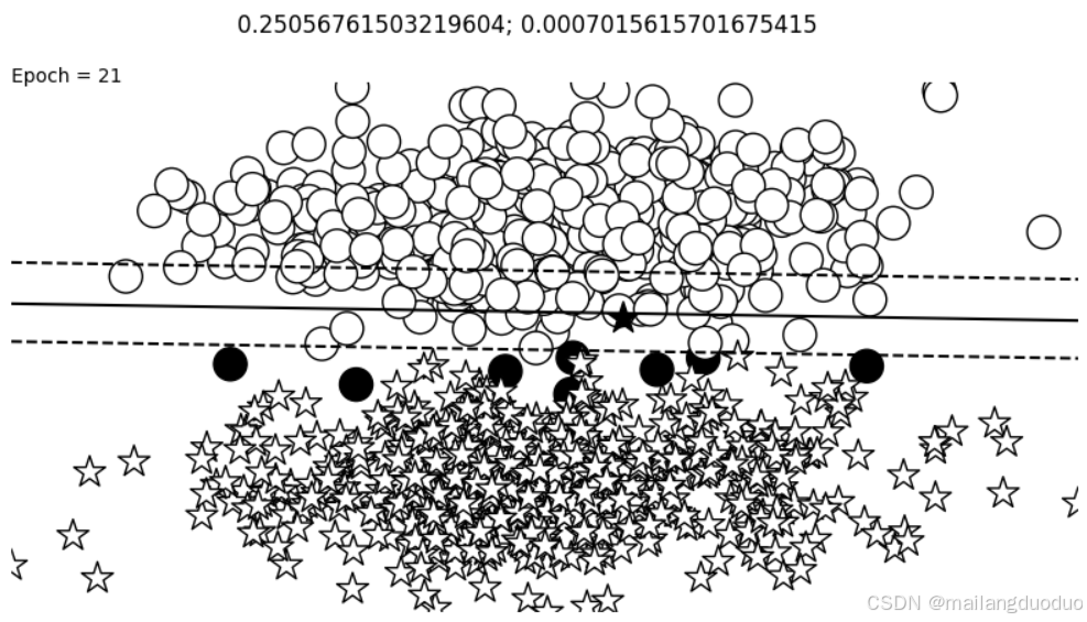


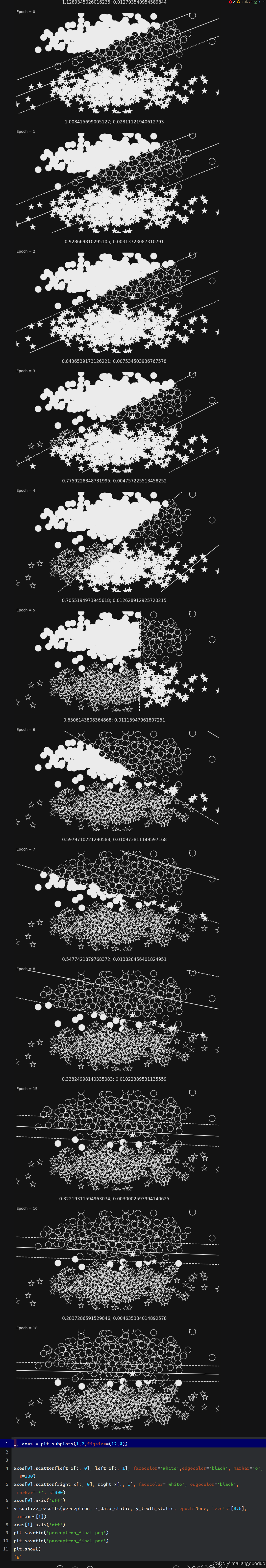
这里之所以和之前的颜色设置的不太一样，是因为主题选择有关

5.结语

本案例至此介绍完毕，主要是感知机模型，使用的自制数据集，实现了简单的二分类问题。如有不足欢迎批评指出！！！