一、参数规模的基本概念

1.1 什么是模型参数？

模型参数是神经网络在训练过程中学习的权重和偏置，它们决定了模型如何处理输入数据并生成输出。

参数类型示例：

# 神经网络中的参数示例
class SimpleNeuralNetwork:
    def __init__(self, input_size, hidden_size, output_size):
        # 权重参数 - 连接不同层之间的强度
        self.w1 = torch.randn(input_size, hidden_size)  # 参数1
        self.b1 = torch.randn(hidden_size)              # 参数2
        self.w2 = torch.randn(hidden_size, output_size) # 参数3
        self.b2 = torch.randn(output_size)              # 参数4
        
    def count_parameters(self):
        # 计算总参数数量
        total = self.w1.numel() + self.b1.numel() + \
                self.w2.numel() + self.b2.numel()
        return total

# 一个小型网络的参数计算
model = SimpleNeuralNetwork(1000, 2000, 500)
print(f"参数数量: {model.count_parameters():,}")  # 约 2.5M 参数

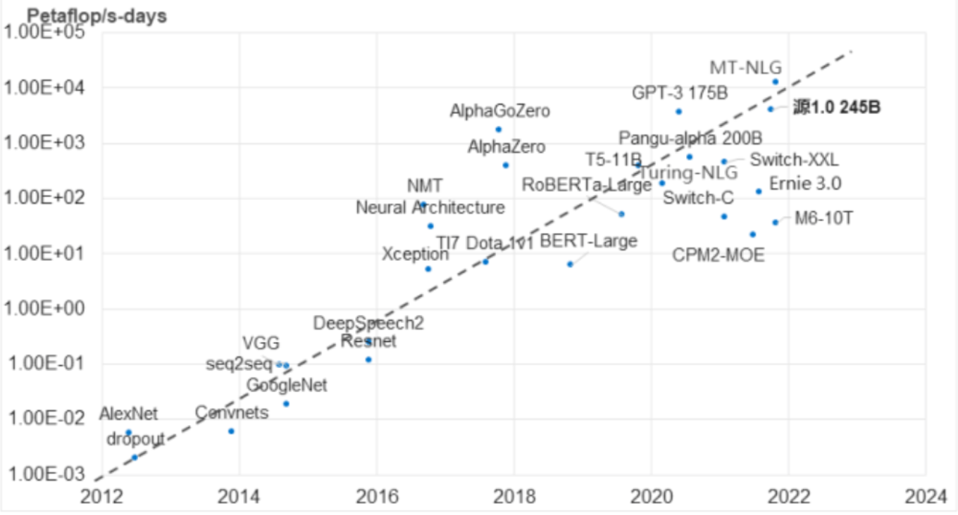
1.2 参数规模的发展历程

参数规模演进时间线：

年代	代表模型	参数量	相当于
2018	BERT-base	1.1亿	一本长篇小说的文本量
2019	GPT-2	15亿	一个小型图书馆
2020	GPT-3	1750亿	一个大型国家图书馆
2023	GPT-4	~1.8万亿	所有印刷文字的总和

二、千亿级参数详解

2.1 千亿参数的技术含义

计算千亿参数的物理意义：

# 千亿参数(1000亿 = 100,000,000,000)的直观理解
billion_params = 100_000_000_000

# 存储需求
storage_gb = (billion_params * 4) / (1024**3)  # FP32精度
print(f"FP32存储需求: {storage_gb:.1f} GB")

# 如果使用FP16精度
storage_gb_fp16 = (billion_params * 2) / (1024**3)
print(f"FP16存储需求: {storage_gb_fp16:.1f} GB")

# 训练数据量关系
training_tokens = 300 * billion_params  # Chinchilla定律
print(f"理想训练token数: {training_tokens:,}")

千亿参数模型的典型特征：

• 需要 200-400GB 显存进行推理
• 训练数据量：2-4万亿 tokens
• 训练成本：数百万美元
• 涌现能力开始出现

2.2 千亿级模型的架构组成

# 千亿参数模型的典型架构分解
class HundredBillionModel:
    def __init__(self):
        self.config = {
            "hidden_size": 12288,      # 12K隐藏维度
            "num_layers": 96,          # 96个Transformer层
            "num_attention_heads": 96, # 96个注意力头
            "vocab_size": 100000,      # 10万词汇表
        }
    
    def calculate_parameters(self):
        # 嵌入层参数
        embedding_params = self.config["vocab_size"] * self.config["hidden_size"]
        
        # Transformer层参数（每层）
        layer_params = (
            # 注意力层: QKV投影 + 输出投影
            4 * self.config["hidden_size"] * self.config["hidden_size"] +
            # 前馈网络: 两个线性层（通常hidden_size * 4）
            2 * self.config["hidden_size"] * (4 * self.config["hidden_size"]) +
            # 层归一化参数（可忽略）
            2 * self.config["hidden_size"]
        )
        
        total_params = embedding_params + self.config["num_layers"] * layer_params
        return total_params

model = HundredBillionModel()
print(f"估计参数量: {model.calculate_parameters():,}")

三、万亿级参数的技术挑战

3.1 万亿参数的物理挑战

存储和内存需求：

# 万亿参数(1,000,000,000,000)的存储分析
trillion_params = 1_000_000_000_000

# 不同精度下的存储需求
precisions = {
    "FP32": 4,
    "FP16": 2, 
    "INT8": 1,
    "INT4": 0.5
}

print("万亿参数存储需求:")
for precision, bytes_per_param in precisions.items():
    storage_tb = (trillion_params * bytes_per_param) / (1024**4)
    print(f"{precision}: {storage_tb:.1f} TB")

# 内存带宽需求
memory_bandwidth = (trillion_params * 2) / (1024**4)  # 每次推理的字节数
print(f"单次推理内存访问量: {memory_bandwidth:.1f} TB")

万亿级模型的现实约束：

• 单个GPU无法容纳整个模型
• 需要复杂的模型并行策略
• 通信开销成为瓶颈
• 能源消耗极其巨大

3.2 分布式训练策略

# 模型并行策略示例
class TrillionParameterTraining:
    def __init__(self):
        self.num_gpus = 512  # 需要的GPU数量
        self.model_shards = 64  # 模型分片数量
        
    def training_requirements(self):
        requirements = {
            "GPU内存总量": f"{self.num_gpus * 80} GB",  # 假设每卡80GB
            "模型分片": self.model_shards,
            "通信带宽": "> 800 Gbps",
            "训练时间": "数周到数月",
            "电力消耗": "兆瓦级别"
        }
        return requirements

training = TrillionParameterTraining()
for key, value in training.training_requirements().items():
    print(f"{key}: {value}")

四、参数规模与模型能力的关系

4.1 缩放定律

Kaplan缩放定律：

模型性能 ∝ (参数数量)^α × (训练数据量)^β × (计算量)^γ

Chinchilla定律的优化：

def chinchilla_optimal_allocation(compute_budget):
    """
    根据计算预算确定最优的参数数量和训练数据量
    """
    # Chinchilla定律：模型参数和训练数据应该平衡
    optimal_params = 20 * (compute_budget ** 0.5)  # 简化公式
    optimal_tokens = 20 * (compute_budget ** 0.5)
    
    return {
        "optimal_parameters": f"{optimal_params:.0f}B",
        "optimal_training_tokens": f"{optimal_tokens:.0f}B",
        "compute_budget": f"{compute_budget:.2e} FLOPs"
    }

# 不同计算预算下的最优配置
budgets = [1e18, 1e21, 1e24]  # FLOPs
for budget in budgets:
    config = chinchilla_optimal_allocation(budget)
    print(config)

4.2 涌现能力

参数规模触发的质变：

涌现能力的具体表现：

• 上下文学习：从少量示例中学习新任务
• 指令跟随：理解并执行自然语言指令
• 思维链：进行多步推理并展示思考过程
• 代码生成：编写、调试和解释程序代码

五、计算成本分析

5.1 训练成本分解

class TrainingCostCalculator:
    def __init__(self, parameters, training_tokens):
        self.parameters = parameters
        self.training_tokens = training_tokens
        
    def compute_flops(self):
        # 训练FLOPs ≈ 6 * 参数数量 * 训练tokens
        return 6 * self.parameters * self.training_tokens
    
    def estimate_cost(self, flops_per_dollar=1e15):
        """估计训练成本（简化计算）"""
        total_flops = self.compute_flops()
        cost_dollars = total_flops / flops_per_dollar
        
        # GPU时间估算（假设A100性能）
        a100_flops = 312e12  # A100 FP16 Tensor Core
        gpu_hours = total_flops / (a100_flops * 3600)
        gpu_years = gpu_hours / (24 * 365)
        
        return {
            "total_flops": f"{total_flops:.2e}",
            "estimated_cost": f"${cost_dollars:,.0f}",
            "gpu_years": f"{gpu_years:,.1f}",
            "gpu_count_1_month": f"{gpu_years * 12:.0f}"
        }

# 不同规模模型的训练成本
models = {
    "GPT-3 (175B)": TrainingCostCalculator(175e9, 300e9),
    "Hypothetical 1T": TrainingCostCalculator(1e12, 2e12),
    "Hypothetical 10T": TrainingCostCalculator(10e12, 20e12)
}

for name, calculator in models.items():
    print(f"\n{name}:")
    for key, value in calculator.estimate_cost().items():
        print(f"  {key}: {value}")

5.2 推理成本分析

class InferenceCostAnalyzer:
    def __init__(self, parameters, context_length=2048):
        self.parameters = parameters
        self.context_length = context_length
        
    def memory_requirements(self):
        """推理内存需求"""
        # 模型权重 + KV缓存
        model_memory_gb = (self.parameters * 2) / (1024**3)  # FP16
        kv_cache_gb = (2 * self.parameters * self.context_length * 2) / (1024**3)
        
        return {
            "model_weights": f"{model_memory_gb:.1f} GB",
            "kv_cache": f"{kv_cache_gb:.1f} GB",
            "total_memory": f"{model_memory_gb + kv_cache_gb:.1f} GB"
        }
    
    def throughput_analysis(self, tokens_per_second=100):
        """吞吐量分析"""
        tokens_per_day = tokens_per_second * 3600 * 24
        cost_per_million_tokens = 10  # 假设成本
        
        return {
            "daily_throughput": f"{tokens_per_day:,} tokens",
            "cost_per_million": f"${cost_per_million_tokens}",
            "daily_revenue_10k_users": f"${tokens_per_day * cost_per_million_tokens / 1e6 * 10000:.0f}"
        }

# 不同规模模型的推理需求
analyzer_100b = InferenceCostAnalyzer(100e9)
analyzer_1t = InferenceCostAnalyzer(1e12)

print("100B模型推理需求:")
for key, value in analyzer_100b.memory_requirements().items():
    print(f"  {key}: {value}")

print("\n1T模型推理需求:")  
for key, value in analyzer_1t.memory_requirements().items():
    print(f"  {key}: {value}")

六、参数效率与模型优化

6.1 混合专家模型

class MixtureOfExperts:
    def __init__(self, total_parameters, num_experts, expert_capacity):
        self.total_parameters = total_parameters
        self.num_experts = num_experts
        self.expert_capacity = expert_capacity
        
    def analyze_efficiency(self):
        """分析MoE的效率优势"""
        # 传统稠密模型参数
        dense_params = self.total_parameters
        
        # MoE模型参数（每个专家有total_parameters/num_experts参数）
        params_per_expert = self.total_parameters / self.num_experts
        active_params_per_token = params_per_expert * self.expert_capacity
        
        efficiency_ratio = dense_params / active_params_per_token
        
        return {
            "total_parameters": f"{self.total_parameters:.0e}",
            "active_parameters_per_token": f"{active_params_per_token:.0e}",
            "efficiency_improvement": f"{efficiency_ratio:.1f}x",
            "sparsity": f"{(1 - self.expert_capacity/self.num_experts)*100:.1f}%"
        }

# MoE模型示例
moe_1t = MixtureOfExperts(1e12, num_experts=8, expert_capacity=2)
print("1万亿参数MoE模型分析:")
for key, value in moe_1t.analyze_efficiency().items():
    print(f"  {key}: {value}")

6.2 模型压缩技术

量化与蒸馏：

class ModelCompression:
    def __init__(self, original_parameters):
        self.original_parameters = original_parameters
        
    def compression_techniques(self):
        techniques = {
            "FP32 → FP16": 0.5,      # 2倍压缩
            "FP16 → INT8": 0.5,      # 2倍压缩  
            "INT8 → INT4": 0.5,      # 2倍压缩
            "Pruning (50%)": 0.5,    # 2倍压缩
            "Distillation (小模型)": 0.1  # 10倍压缩
        }
        
        results = {}
        current_size = self.original_parameters
        for technique, ratio in techniques.items():
            current_size *= ratio
            results[technique] = f"{current_size:.2e} params"
            
        return results

compression = ModelCompression(1e12)
print("1万亿参数模型的压缩潜力:")
for technique, size in compression.compression_techniques().items():
    print(f"  {technique}: {size}")

七、实际影响与应用

7.1 硬件需求演进

GPU内存发展轨迹：

2018: V100 16GB → 可训练 1B 模型
2020: A100 40GB → 可训练 10B 模型  
2022: A100 80GB → 可训练 50B 模型
2024: H100 80GB → 可训练 100B+ 模型
未来: 需要 1TB+ 内存单卡支持万亿模型

7.2 实际部署考虑

class DeploymentConsiderations:
    def __init__(self, parameters, qps_requirement=1000):
        self.parameters = parameters
        self.qps = qps_requirement
        
    def infrastructure_needs(self):
        """基础设施需求估算"""
        # 内存需求
        memory_per_instance_gb = (self.parameters * 2) / (1024**3)  # FP16
        
        # 计算需求（简化估算）
        flops_per_token = 2 * self.parameters  # 每token的FLOPs
        total_flops_needed = flops_per_token * self.qps
        
        # GPU数量估算（假设A100）
        a100_performance = 312e12  # FLOPs/s
        gpus_needed = total_flops_needed / a100_performance
        
        return {
            "memory_per_instance": f"{memory_per_instance_gb:.0f} GB",
            "gpus_for_target_qps": f"{gpus_needed:.1f}",
            "estimated_power_consumption": f"{gpus_needed * 0.4:.1f} kW",
            "monthly_cloud_cost": f"${gpus_needed * 5 * 24 * 30:,.0f}"  # $5/GPU-hour
        }

deployment_100b = DeploymentConsiderations(100e9)
print("100B模型部署需求:")
for key, value in deployment_100b.infrastructure_needs().items():
    print(f"  {key}: {value}")

八、未来发展趋势

8.1 参数规模的物理极限

可能的技术突破：

• 光学计算和量子计算
• 神经形态计算芯片
• 更高效的模型架构
• 算法层面的根本创新

8.2 参数效率的优化方向

class FutureTrends:
    @staticmethod
    def parameter_efficiency_roadmap():
        trends = [
            {
                "阶段": "当前",
                "重点": "规模扩展", 
                "关键技术": ["混合专家", "模型并行", "量化"],
                "参数规模": "1-10万亿"
            },
            {
                "阶段": "近期(2-3年)", 
                "重点": "效率优化",
                "关键技术": ["算法创新", "硬件协同设计", "动态网络"],
                "参数规模": "10-100万亿"
            },
            {
                "阶段": "长期(5年+)",
                "重点": "质变突破", 
                "关键技术": ["新计算范式", "生物启发", "量子混合"],
                "参数规模": "100万亿+"
            }
        ]
        return trends

trends = FutureTrends.parameter_efficiency_roadmap()
for trend in trends:
    print(f"\n{trend['阶段']}:")
    print(f"  重点: {trend['重点']}")
    print(f"  关键技术: {', '.join(trend['关键技术'])}")
    print(f"  参数规模: {trend['参数规模']}")

九、总结与启示

9.1 核心要点总结

千亿级参数意味着：

• 模型具备了涌现能力和复杂推理能力
• 训练和部署成本达到百万美元级别
• 需要大规模分布式计算基础设施
• 开始触及当前硬件的物理极限

万亿级参数意味着：

• 可能需要重新思考神经网络架构
• 催生新的计算硬件和算法
• 模型能力可能产生质的飞跃
• 对社会各行业的颠覆性影响

9.2 技术发展启示

关键认知：

1. 参数不是万能的：需要与数据、算法、架构平衡发展
2. 效率至关重要：未来的竞争在于单位参数的性能
3. 硬件算法协同：需要从系统层面优化整个技术栈
4. 普惠化是方向：最终目标是让强大AI能力人人可用

千亿级和万亿级参数不仅代表了技术的进步，更标志着人工智能正在从实验室走向现实世界，从工具性技术走向基础设施性技术的重要转折点。