• 🍨 本文为🔗365天深度学习训练营 中的学习记录博客
• 🍖 原作者：K同学啊

1. 简介 & 数据集介绍

本实验使用 ResNet50 深度残差网络对眼底图像进行三分类（Normal / Mild / Severe），实现视网膜病变严重程度的自动分级。数据集共 1661 张图像，按 80/20 划分为训练集和测试集，以 ImageNet 预训练的均值和标准差做归一化，使用 AdamW 优化器和交叉熵损失进行端到端训练。

ResNet（Residual Network）由微软研究院何恺明等人于 2015 年提出，核心思想是引入残差连接（Skip Connection） 解决深层网络的退化问题。传统网络层数加深后，训练误差反而上升。ResNet 让网络学习残差映射 $F(x)=H(x)-x$，而非直接学习 $H(x)$，使得梯度可以通过 shortcut 直接回传，大幅缓解了梯度消失。ResNet50 采用 Bottleneck 结构，每个残差块包含三层：1×1 降维 → 3×3 卷积 → 1×1 升维。网络共 5 个阶段，逐步将特征图从 224×224 缩小到 7×7，通道数从 64 扩展到 2048，最终通过全局平均池化和全连接层输出分类结果。

2. 环境

• 语言环境：Python 3.14.6
• 编译器：Jupyter Notebook
• 深度学习环境：PyTorch ( torch 2.12.1 + torchvision 0.27.1 )

3. 代码实现

3.1 前期准备

3.1.1 设置GPU & 导入库

导入 PyTorch、torchvision 等深度学习库，配置 matplotlib 中文字体，自动选择 GPU/CPU 设备.

import torch
import torch.nn as nn
from torchvision import transforms, datasets
import os, PIL, pathlib, warnings
import torchsummary as summary
import copy
import matplotlib.pyplot as plt
from PIL import Image
from datetime import datetime

warnings.filterwarnings("ignore")
plt.rcParams["figure.dpi"] = 100
plt.rcParams['font.sans-serif'] = ['SimHei']
plt.rcParams['axes.unicode_minus'] = False

device = torch.device("cuda" if torch.cuda.is_available() else "cpu")
device

3.1.2 可视化样本图片

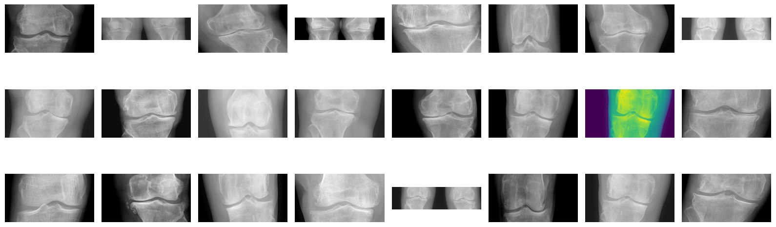
从 “2Mild” 类别中读取图片并用 matplotlib 展示，用于直观了解数据内容和质量。

image_folder='./Data/data/2Mild/'
image_files = [f for f in os. listdir(image_folder) if f.endswith((".jpg", ".png", ".jpeg"))]
fig, axes = plt.subplots(3, 8, figsize=(16, 6))

for ax, img_file in zip(axes.flat, image_files):
    img_path = os.path.join(image_folder, img_file)
    img = Image.open(img_path)
    ax.imshow(img)
    ax.axis('off')

plt.tight_layout()
plt.show()

3.2 数据预处理

3.2.1 加载数据集并定义预处理

使用 ImageFolder 加载数据，定义图像预处理流程：缩放到 224×224 → 转为 Tensor → 用 ImageNet 均值和标准差做归一化。

data_dir = './Data/data/'

train_transforms = transforms.Compose([
    transforms.Resize((224, 224)),
    transforms.ToTensor(),
    transforms.Normalize(mean=[0.485, 0.456, 0.406], std=[0.229, 0.224, 0.225])
])

total_data = datasets.ImageFolder(data_dir, transform=train_transforms)
total_data

Dataset ImageFolder
    Number of datapoints: 1661
    Root location: ./Data/data/
    StandardTransform
Transform: Compose(
               Resize(size=(224, 224), interpolation=bilinear, max_size=None, antialias=True)
               ToTensor()
               Normalize(mean=[0.485, 0.456, 0.406], std=[0.229, 0.224, 0.225])
           )

3.2.2 查看类别映射

查看 ImageFolder 自动分配的类别标签与索引的对应关系。可以看到三个类别分别映射到 0、1、2。

total_data.class_to_idx

{'0Normal': 0, '2Mild': 1, '4Severe': 2}

3.2.3 划分训练集和测试集

按 80/20 比例将数据随机划分为训练集和测试集，用于模型训练和评估。

train_size = int(0.8*len(total_data))
test_size = len(total_data) - train_size
train_dataset, test_dataset = torch.utils.data.random_split(total_data, [train_size, test_size])
train_dataset, test_dataset

(<torch.utils.data.dataset.Subset at 0x118e65400>,
 <torch.utils.data.dataset.Subset at 0x118deb110>)

3.2.4 创建 DataLoader

将数据集封装为 DataLoader，训练集打乱顺序（shuffle=True），测试集不打乱。打印一个 batch 的形状确认数据格式正确。

batch_size = 4
train_dl = torch.utils.data.DataLoader(train_dataset, batch_size=batch_size, shuffle=True)
test_dl = torch.utils.data.DataLoader(test_dataset, batch_size=batch_size)

for X, y in test_dl:
    print("Shape of X [N, C, H, W]: ", X.shape)
    print("Shape of y: ", y.shape, y.dtype)
    break

Shape of X [N, C, H, W]:  torch.Size([4, 3, 224, 224])
Shape of y:  torch.Size([4]) torch.int64

3.3 模型建立与训练

3.3.1 定义 ResNet50 模型

手动实现 ResNet50 网络，包含：

• IdentityBlock：残差块，输入输出尺寸相同，用于堆叠同维度的卷积层
• ConvBlock：带下采样的残差块，通过 stride=2 降低特征图尺寸，同时用 1x1 卷积调整 shortcut 的通道数
• ResNet50：完整的 50 层网络，最后通过平均池化和全连接层输出 3 分类结果.

def autopad(k, p=None):
    if p is None:
        if isinstance(k, int):
            p = k // 2
        else:
            p = [x // 2 for x in k]
    return p

class IdentityBlock(nn.Module):
    def __init__(self, in_channels, kernel_size, filters):
        super(IdentityBlock, self).__init__()
        filters1, filters2, filters3 = filters
        self.conv1 = nn.Sequential(nn.Conv2d(in_channels, filters1, 1, stride=1, padding=0, bias=False), nn.BatchNorm2d(filters1), nn.ReLU())
        self.conv2 = nn.Sequential(nn.Conv2d(filters1, filters2, kernel_size, stride=1, padding=autopad(kernel_size), bias=False), nn.BatchNorm2d(filters2), nn.ReLU())
        self.conv3 = nn.Sequential(nn.Conv2d(filters2, filters3, 1, stride=1, padding=0, bias=False), nn.BatchNorm2d(filters3))
        self.relu = nn.ReLU()

    def forward(self, x):
        x1 = self.conv1(x)
        x1 = self.conv2(x1)
        x1 = self.conv3(x1)
        x = x + x1
        x = self.relu(x)
        return x
    
class ConvBlock(nn.Module):
    def __init__(self, in_channels, kernel_size, filters, stride=2):
        super(ConvBlock, self).__init__()
        filters1, filters2, filters3 = filters
        self.conv1 = nn.Sequential(nn.Conv2d(in_channels, filters1, 1, stride=stride, padding=0, bias=False), nn.BatchNorm2d(filters1), nn.ReLU())
        self.conv2 = nn.Sequential(nn.Conv2d(filters1, filters2, kernel_size, stride=1, padding=autopad(kernel_size), bias=False), nn.BatchNorm2d(filters2), nn.ReLU())
        self.conv3 = nn.Sequential(nn.Conv2d(filters2, filters3, 1, stride=1, padding=0, bias=False), nn.BatchNorm2d(filters3))
        self.conv4 = nn.Sequential(nn.Conv2d(in_channels, filters3, 1, stride=stride, padding=0, bias=False), nn.BatchNorm2d(filters3))
        self.relu = nn.ReLU()

    def forward(self, x):
        x1 = self.conv1(x)
        x1 = self.conv2(x1)
        x1 = self.conv3(x1)
        x2 = self.conv4(x)
        x = x1 + x2
        x = self.relu(x)
        return x
    
class ResNet50(nn.Module):
    def __init__(self, classes=1000):
        super(ResNet50, self).__init__()
        self.conv1 = nn.Sequential(nn.Conv2d(3, 64, 7, stride=2, padding=3, bias=False, padding_mode='zeros'), nn.BatchNorm2d(64), nn.ReLU(), nn.MaxPool2d(kernel_size=3, stride=2, padding=1))
        self.conv2 = nn.Sequential(ConvBlock(64, 3, [64, 64, 256], stride=1), IdentityBlock(256, 3, [64, 64, 256]),IdentityBlock(256, 3, [64, 64, 256]))
        self.conv3 = nn.Sequential(ConvBlock(256, 3, [128, 128, 512]),IdentityBlock(512, 3, [128, 128, 512]),IdentityBlock(512, 3, [128, 128, 512]),IdentityBlock(512, 3, [128, 128, 512]))
        self.conv4 = nn.Sequential(ConvBlock(512, 3, [256, 256, 1024]),IdentityBlock(1024, 3, [256, 256, 1024]),IdentityBlock(1024, 3, [256, 256, 1024]), IdentityBlock(1024,3,[256, 256, 1024]), IdentityBlock(1024,3,[256,256,1024]), IdentityBlock(1024,3,[256,256,1024]))
        self.conv5 = nn.Sequential(ConvBlock(1024, 3, [512, 512, 2048]), IdentityBlock(2048,3,[512, 512,2048]))
        self.pool = nn.AvgPool2d(kernel_size=7, stride=7, padding=0)
        self.fc = nn.Linear(2048, 3)

    def forward(self,x):
        x = self.conv1(x)
        x = self.conv2(x)
        x = self.conv3(x)
        x = self.conv4(x)
        x = self.conv5(x)
        x = self.pool(x)
        x = torch.flatten(x, start_dim=1)
        x = self.fc(x)
        return x

model = ResNet50().to(device)
model

ResNet50(
  (conv1): Sequential(
    (0): Conv2d(3, 64, kernel_size=(7, 7), stride=(2, 2), padding=(3, 3), bias=False)
    (1): BatchNorm2d(64, eps=1e-05, momentum=0.1, affine=True, bias=True, track_running_stats=True)
    (2): ReLU()
    (3): MaxPool2d(kernel_size=3, stride=2, padding=1, dilation=1, ceil_mode=False)
  )
  (conv2): Sequential(
    (0): ConvBlock(
      (conv1): Sequential(
        (0): Conv2d(64, 64, kernel_size=(1, 1), stride=(1, 1), bias=False)
        (1): BatchNorm2d(64, eps=1e-05, momentum=0.1, affine=True, bias=True, track_running_stats=True)
        (2): ReLU()
      )
      (conv2): Sequential(
        (0): Conv2d(64, 64, kernel_size=(3, 3), stride=(1, 1), padding=(1, 1), bias=False)
        (1): BatchNorm2d(64, eps=1e-05, momentum=0.1, affine=True, bias=True, track_running_stats=True)
        (2): ReLU()
      )
      (conv3): Sequential(
        (0): Conv2d(64, 256, kernel_size=(1, 1), stride=(1, 1), bias=False)
        (1): BatchNorm2d(256, eps=1e-05, momentum=0.1, affine=True, bias=True, track_running_stats=True)
      )
      (conv4): Sequential(
        (0): Conv2d(64, 256, kernel_size=(1, 1), stride=(1, 1), bias=False)
...
    )
  )
  (pool): AvgPool2d(kernel_size=7, stride=7, padding=0)
  (fc): Linear(in_features=2048, out_features=3, bias=True)
)

3.3.2 模型结构概览

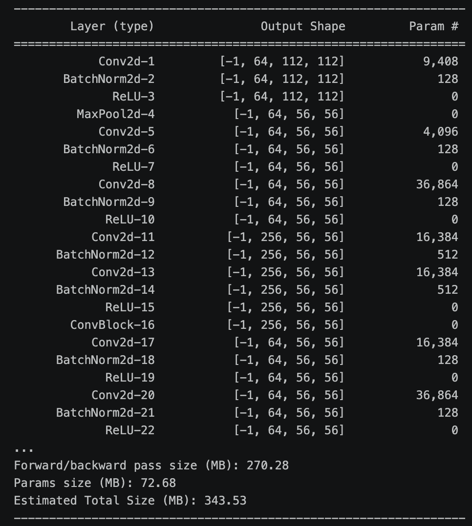
使用 torchsummary 打印模型每层的输出形状和参数量，便于确认网络结构是否正确搭建。

summary.summary(model, (3, 224, 224))

3.3.3 定义训练和测试函数

• train()：遍历训练集，前向传播 → 计算损失 → 反向传播 → 更新参数，累计损失和正确预测数
• test()：在 torch.no_grad() 下遍历测试集，只做前向传播，不更新梯度

def train(dataloader, model, loss_fn, optimizer):
    size = len(dataloader.dataset)
    num_batches = len(dataloader)

    train_loss, train_acc = 0, 0

    for X, y in dataloader:
        X, y = X.to(device), y.to(device)

        pred = model(X)
        loss = loss_fn(pred, y)

        optimizer.zero_grad()
        loss.backward()
        optimizer.step()

        train_loss += loss.item()
        train_acc += (pred.argmax(1) == y).type(torch.float).sum().item()

    train_loss /= num_batches
    train_acc /= size

    return train_loss, train_acc

def test(dataloader, model, loss_fn):
    size = len(dataloader.dataset)
    num_batches = len(dataloader)

    test_loss, test_acc = 0, 0

    with torch.no_grad():
        for imgs, target in dataloader:
            imgs, target = imgs.to(device), target.to(device)

            target_pred = model(imgs)
            loss = loss_fn(target_pred, target)

            test_acc += (target_pred.argmax(1) == target).type(torch.float).sum().item()
            test_loss += loss.item()

    test_loss /= num_batches
    test_acc /= size

    return test_loss, test_acc

3.3.4 训练模型

定义优化器（AdamW）、损失函数（交叉熵），进行 10 个 epoch 的训练。每个 epoch 结束后在测试集上评估，保存最优模型权重。

optimizer = torch.optim.AdamW(model.parameters(), lr=1e-4)
loss_fn = nn.CrossEntropyLoss()

epochs = 10

train_loss, train_acc = [], []
test_loss, test_acc = [], []

best_acc = 0

for epoch in range(epochs):
    model.train()
    train_epoch_acc, train_epoch_loss = train(train_dl, model, loss_fn, optimizer)

    model.eval()
    epoch_test_acc, epoch_test_loss = test(test_dl, model, loss_fn)

    if epoch_test_acc > best_acc:
        best_acc = epoch_test_acc
        best_model_wts = copy.deepcopy(model)

    train_acc.append(train_epoch_acc)
    train_loss.append(train_epoch_loss)
    test_acc.append(epoch_test_acc)
    test_loss.append(epoch_test_loss)

    lr = optimizer.param_groups[0]['lr']
    template = ("Epoch: {:2d}, Train_acc: {:.1f}%, Train_loss: {:.3f}, Test_acc: {:.1f}%, Test_loss: {:.3f}, Lr: {:.2E}")
    print(template.format(epoch+1, train_epoch_acc*100, train_epoch_loss, epoch_test_acc*100, epoch_test_loss, lr))

PATH = './best_resnet50.pth'
torch.save(best_model_wts.state_dict(), PATH)

print('Done.')

Epoch:  1, Train_acc: 88.1%, Train_loss: 0.643, Test_acc: 78.5%, Test_loss: 0.694, Lr: 1.00E-04
Epoch:  2, Train_acc: 68.2%, Train_loss: 0.735, Test_acc: 78.1%, Test_loss: 0.736, Lr: 1.00E-04
Epoch:  3, Train_acc: 54.6%, Train_loss: 0.811, Test_acc: 52.8%, Test_loss: 0.787, Lr: 1.00E-04
Epoch:  4, Train_acc: 48.0%, Train_loss: 0.820, Test_acc: 59.0%, Test_loss: 0.781, Lr: 1.00E-04
Epoch:  5, Train_acc: 44.0%, Train_loss: 0.838, Test_acc: 44.5%, Test_loss: 0.844, Lr: 1.00E-04
Epoch:  6, Train_acc: 37.8%, Train_loss: 0.863, Test_acc: 42.7%, Test_loss: 0.853, Lr: 1.00E-04
Epoch:  7, Train_acc: 36.8%, Train_loss: 0.860, Test_acc: 33.3%, Test_loss: 0.871, Lr: 1.00E-04
Epoch:  8, Train_acc: 32.0%, Train_loss: 0.884, Test_acc: 69.7%, Test_loss: 0.763, Lr: 1.00E-04
Epoch:  9, Train_acc: 34.7%, Train_loss: 0.867, Test_acc: 35.0%, Test_loss: 0.871, Lr: 1.00E-04
Epoch: 10, Train_acc: 25.6%, Train_loss: 0.913, Test_acc: 31.2%, Test_loss: 0.892, Lr: 1.00E-04
Done.

4. 不同优化器对比评估

4.1 可视化训练过程

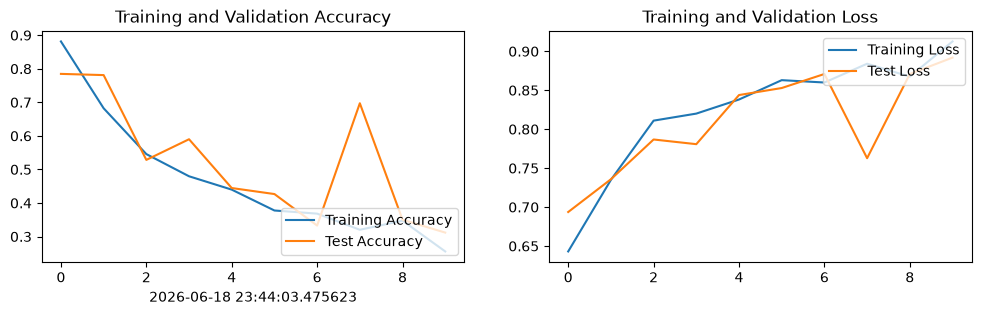
绘制训练和测试的准确率、损失曲线，并使用 Matplotlib 将训练集与验证集的准确率（Accuracy）和损失值（Loss）随时间变化的趋势绘制成了两幅直观的折线图。

current_time = datetime.now()

epochs_range = range(epochs)

plt.figure(figsize=(12, 3))
plt.subplot(1, 2, 1)

plt.plot(epochs_range, train_acc, label='Training Accuracy')
plt.plot(epochs_range, test_acc, label='Test Accuracy')
plt.legend(loc='lower right')
plt.title('Training and Validation Accuracy')
plt.xlabel(current_time)

plt.subplot(1, 2, 2)
plt.plot(epochs_range, train_loss, label='Training Loss')
plt.plot(epochs_range, test_loss, label='Test Loss')
plt.legend(loc='upper right')
plt.title('Training and Validation Loss')
plt.show()

4.2 加载最优模型并评估

加载训练过程中保存的最优模型权重，在测试集上进行最终评估，输出测试准确率和损失值。

best_model_wts.load_state_dict(torch.load(PATH, map_location=device))
test_epoch_acc, test_epoch_loss = test(test_dl, best_model_wts, loss_fn)
test_epoch_acc, test_epoch_loss

(0.7847635056380005, 0.6936936936936937)