一、前言

仅供参考，未经实验验证。 作者提到强化学习的作用是让模型的输出分布更稳定、更一致——把原本散落在 TopK 中的正确答案"集中"到最可能的那个答案上，并没有增强模型"生成正确答案的基本能力" 。此外，在附录中用数学公式说明了强化学习的SFT、RFT、DPO、PPO、GRPO统一范式

二、DeepSeekMath

论文标题： DeepSeekMath: Pushing the Limits of Mathematical Reasoning in Open Language Models
（DeepSeekMath：推动开放语言模型中数学推理的极限）
作者： Zhihong Shao, Peiyi Wang, Qihao Zhu, Runxin Xu, Junxiao Song, Mingchuan Zhang, Y.K. Li, Y. Wu, Daya Guo
机构： DeepSeek-AI（主导）、清华大学、北京大学
发表时间： 2024年2月6日（arXiv:2402.03300）
GitHub： https://github.com/deepseek-ai/DeepSeek-Math
论文地址： https://arxiv.org/pdf/2402.03300

5. 讨论

为什么强化学习有效？

In this paper, we conduct reinforcement learning based on a subset of instruction tuning data, and it achieves significant performance enhancement upon the instruction tuning model. To further explain why reinforcement learning works. We evaluate the Pass@K and Maj@K accuracy of the Instruct and RL models on two benchmarks.
本文基于指令微调数据的一个子集进行了强化学习，并在指令微调模型上实现了显著的性能提升。为了进一步解释强化学习为何有效。我们在两个基准测试上评估了Instruct模型和RL模型的Pass@K和Maj@K准确率。
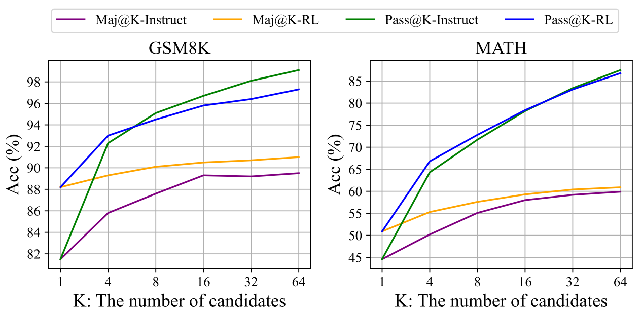Figure 7 | The Maj@K and Pass@K of SFT and RL DeepSeekMath 7B on GSM8K and MATH (temperature 0.7). It was noted that RL enhances Maj@K but not Pass@K.
图7 SFT 和 RL 版本的 DeepSeekMath 7B 在 GSM8K 和 MATH 上的 Maj@K 和 Pass@K 指标（采样温度 0.7）。可以观察到，RL 提升了 Maj@K，但并未提升 Pass@K。

---

补充解释这两个指标：

• Pass@K：同一道题让模型采样生成 K 次，只要这 K 次里至少有一次答对，就算通过。它衡量的是模型的**“潜力”**——有没有能力生成正确答案。
• Maj@K：同一道题采样生成 K 次，然后对这 K 个答案做多数投票（选出现次数最多的答案），看这个最终答案是否正确。它衡量的是模型的**“稳定性/一致性”**——最可能给出的答案是不是对的。

这句话的言外之意：RL 训练让模型更稳定、更一致了（多数投票结果更好），但并没有扩大模型生成正确答案的覆盖范围（K 次里能碰对的次数没增加）。说明 RL 主要提升了"答案的一致性"，而不是"探索到更多正确解的能力"。

As shown in Figure 7, RL enhances Maj@K’s performance but not Pass@K. These findings indicate that RL enhances the model’s overall performance by rendering the output distribution more robust, in other words, it seems that the improvement is attributed to boosting the correct response from TopK rather than the enhancement of fundamental capabilities.
如图 7 所示，RL 提升了 Maj@K 的性能，但并未提升 Pass@K 的性能。这些发现表明，RL 通过使输出分布更加鲁棒来提升模型的整体性能，换言之，这种改进似乎归因于提升了 TopK 中的正确响应，而非基础能力的增强。

Similarly, (Wang et al., 2023a) identified a misalignment problem in reasoning tasks within the SFT model, showing that the reasoning performance of SFT models can be improved through a series of preference alignment strategies (Song et al., 2023; Wang et al., 2023a; Yuan et al., 2023b).
类似地，(Wang et al., 2023a) 识别出SFT模型在推理任务中存在不一致问题，并表明通过一系列偏好对齐策略可以提升SFT模型的推理性能 (Song et al., 2023; Wang et al., 2023a; Yuan et al., 2023b).

5.2.3. 如何实现更有效的强化学习？

We demonstrate RL works pretty well in mathematical reasoning tasks. We also provide a unified paradigm to understand different representative training methods. Within this paradigm, all methods are conceptualized as either direct or simplified RL techniques. As summarized in Equation 5, there exist three key components: Data Source, Algorithm, and Reward Function.
我们证明了强化学习在数学推理任务中表现优异。我们还提供了一个统一的范式来理解不同的代表性训练方法。在此范式下，所有方法都被概念化为直接或简化的强化学习技术。如公式 5 总结所示，存在三个关键组成部分：数据源、算法和奖励函数。

We provide some potential future directions about the three components.
我们为这三个组成部分提供了一些潜在的未来发展方向。

Data Source Data source is the raw material of all training methods. In the context of RL, we specifically refer to the data source as the unlabeled questions with the outputs sampled from the policy model. In this paper, we only use the questions from the instruction tuning stage and a naive nucleus sampling to sample outputs.
数据源 训练方法的所有原始材料均来自数据源。在强化学习的背景下，我们特指数据源为来自策略模型的采样输出的未标记问题。在本文中，我们仅使用指令调优阶段的问题，并通过朴素的核采样来采样输出。

We think this is a potential reason that our RL pipeline only improves the Maj@K performance. In the future, we will explore our RL pipeline on out-of-distribution question prompts, in conjunction with advanced sampling (decoding) strategies, like those based on tree-search methods (Yao et al., 2023).
我们认为这是我们强化学习流水线仅能提升Maj@K性能的一个潜在原因。未来，我们将结合基于树搜索方法（Yao et al., 2023）的高级采样（解码）策略，在分布外问题提示上探索我们的强化学习流水线。

Also, the efficient inference techniques (Kwon et al., 2023; Leviathan et al., 2023; Xia et al., 2023, 2024), which determines the exploration efficiency of policy models, also play an exceedingly important role.
此外，高效推理技术（Kwon等人，2023；Leviathan等人，2023；Xia等人，2023，2024)），它决定了策略模型的探索效率，也起着极其重要的作用。策略模型的探索效率，也起着极其重要的作用。

Algorithms Algorithms process the data and reward signal to the gradient coefficient to update the model parameter. Based on Equation 5, to some extent, all methods now fully TRUST the signal of the reward function to increase or decrease the conditional probability of a certain token.
算法 算法处理数据和奖励信号以获得梯度系数来更新模型参数。基于公式 5，在某种程度上，所有方法现在都完全信任奖励函数的信号来增加或减少某个 token 的条件概率。

However, it is impossible to ensure the reward signal is always reliable, especially in extremely complex tasks. For example, even the PRM800K datasets (Lightman et al., 2023), which have been carefully annotated by well-trained annotators, still contain approximately 20% of incorrectly annotations7.
然而，尤其是在极其复杂的任务中，确保奖励信号始终可靠是不可能的。例如，即使是经过精心标注的PRM800K数据集（Lightman等人，2023)），其标注者也经过了良好培训，但仍包含约20%的错误标注7。

To this end, we will explore the reinforcement learning algorithm that is robust against noisy reward signals. We believe such WEAK-TO-STRONG (Burns et al., 2023) alignment methods will bring a fundamental change to the learning algorithms.
为此，我们将探索对噪声奖励信号鲁棒的强化学习算法。我们相信这种 WEAK-TO-STRONG (Burns et al., 2023) 对齐方法将为学习算法带来根本性变革。

Reward Function Reward function is the source of the training signal. In RL, the reward function is usually the neural reward model. We think there exist three important directions for reward models: 1) How to enhance the generalization ability of the reward model. The reward model must be effectively generalized to handle out-of-distribution questions and advanced decoding outputs; otherwise, reinforcement learning may merely stabilize the distribution of LLMs rather than improve their fundamental capabilities; 2) How to reflect the uncertainty of reward model. The uncertainty could potentially act as a linking bridge between the weak reward model and the weak-to-strong learning algorithms; 3) How to efficiently build highquality process reward models that can provide fine-grained training signals for the reasoning process (Lightman et al., 2023; Wang et al., 2023b).
奖励函数 奖励函数是训练信号的来源。在强化学习中，奖励函数通常是神经奖励模型。我们认为奖励模型存在三个重要的研究方向：1) 如何增强奖励模型的泛化能力。奖励模型必须有效地泛化，以处理分布外的提问和高级解码输出；否则，强化学习可能仅仅稳定大型语言模型的分布，而不是提高其基本能力；2) 如何反映奖励模型的不确定性。不确定性可能作为弱奖励模型和由弱到强学习算法之间的桥梁；3) 如何高效地构建高质量的过程奖励模型，从而为推理过程提供细粒度的训练信号（Lightman et al., 2023; Wang et al., 2023b）。

6. 结论、局限与未来工作

We present DeepSeekMath, which outperforms all open-source models on the competitionlevel MATH benchmark and approaches the performance of closed models. DeepSeekMath is initialized with DeepSeek-Coder-v1.5 7B and undergoes continual training for 500B tokens, with a significant component of the training data being 120B math tokens sourced from Common Crawl.
我们提出了DeepSeekMath，它在竞赛级别的MATH基准测试中表现优于所有开源模型，并接近闭源模型的性能。DeepSeekMath使用DeepSeek-Coder-v1.5 7B进行初始化，并经过500B个token的持续训练，其中训练数据的重要组成部分是从Common Crawl获取的120B个数学token。

Our extensive ablation study shows web pages offer significant potential for high-quality mathematical data, while arXiv may not as beneficial as we expected. We introduce Group Relative Policy Optimization (GRPO), a variant of Proximal Policy Optimization (PPO), which can notably improve mathematical reasoning capabilities with less memory consumption.
我们广泛的消融研究表明，网页为高质量的数学数据提供了巨大的潜力，而 arXiv 可能不像我们预期的那样有益。我们引入了群组相对策略优化（GRPO），这是近端策略优化（PPO）的一个变体，它可以在减少内存消耗的同时显著提高数学推理能力。

The experiment results show that GRPO is effective even if DeepSeekMath-Instruct 7B has reached a high score on benchmarks. We also provide a unified paradigm to understand a series of methods and summarize several potential directions for more effective reinforcement learning.
实验结果表明，即使DeepSeekMath-Instruct 7B在基准测试中取得了高分，GRPO仍然有效。我们还提供了一个统一的范式来理解一系列方法，并总结了若干未来更有效的强化学习方向。

Although DeepSeekMath achieves impressive scores on quantitative reasoning benchmarks, its capability on geometry and theorem-proof are relatively weaker than closed models. For instance, in our dry run, the model cannot handle problems related to triangles and ellipses, which may indicate data selection bias in pre-training and fine-tuning.
尽管DeepSeekMath在量化推理基准上取得了令人印象深刻的分数，但其在几何和定理证明方面的能力相对弱于闭源模型。例如，在我们的一次试运行中，该模型无法处理与三角形和椭圆相关的问题，这可能表明预训练和微调中存在数据选择偏差。

In addition, restricted by the model scale, DeepSeekMath is worse than GPT-4 on few-shot capability. GPT-4 could improve its performance with few-shot inputs, while DeepSeekMath shows similar performance in zero-shot and few-shot evaluation. In the future, we will further improve our engineered data selection pipeline to construct more high-quality pre-trained corpus.
此外，受模型规模的限制，DeepSeekMath在少样本能力方面不如GPT-4。GPT-4可以通过少样本输入来提高其性能，而DeepSeekMath在零样本和少样本评估中表现出相似的性能。未来，我们将进一步改进我们工程化的数据选择流程，以构建更高质量的预训练语料库。

In addition, we will explore the potential directions (Section 5.2.3) for more effective reinforcement learning of LLMs.
此外，我们将探讨（第 5.2.3 节）更有效地强化学习大型语言模型的潜在方向。

问题1：总结一下

一、为什么强化学习有效？

论文通过对比 Pass@K 和 Maj@K 两个指标，揭示了 RL 提升性能的真正机制：

• Pass@K：同一题采样 K 次，至少对一次就算通过 → 测模型的**“潜力/覆盖能力”**
• Maj@K：同一题采样 K 次，多数投票后的答案是否正确 → 测模型的**“稳定性/一致性”**

核心发现：RL 显著提升了 Maj@K，但没有提升 Pass@K。这说明：

• RL 并没有增强模型"生成正确答案的基本能力"
• RL 的作用是让模型的输出分布更稳定、更一致——把原本散落在 TopK 中的正确答案"集中"到最可能的那个答案上
• 这本质上是在解决 SFT 模型的**“不一致/错配问题”**（misalignment）

二、如何实现更有效的强化学习？

作者从统一范式的三个组成部分，提出了未来方向：

1. 数据源（Data Source）

• 当前只用了指令微调阶段的问题 + 简单核采样，这可能是 RL 只能提升 Maj@K 的原因
• 未来方向：引入分布外问题（out-of-distribution）和高级采样策略（如树搜索解码），并提升推理效率以改善探索能力

2. 算法（Algorithms）

• 当前所有方法都完全信任奖励信号来调整 token 概率
• 但奖励信号不可能永远可靠（如 PRM800K 仍有约 20% 错误标注）
• 未来方向：探索对噪声奖励鲁棒的算法，引入 Weak-to-Strong 对齐思想

3. 奖励函数（Reward Function）

• 奖励模型是 RL 信号的来源，有三个关键方向：
  1. 增强泛化能力：必须能处理分布外问题和复杂解码输出，否则 RL 只是"稳定分布"而非"提升能力"
  2. 反映不确定性：不确定性可作为弱奖励模型与弱到强学习算法之间的桥梁
  3. 构建高质量过程奖励模型（PRM）：为推理过程提供细粒度、逐步骤的训练信号

三、结论与局限

主要成果：

• DeepSeekMath 在竞赛级 MATH 基准上超越所有开源模型，接近闭源模型
• 基于 DeepSeek-Coder-v1.5 7B，持续训练 500B tokens（含 120B 数学 tokens）
• 提出 GRPO，在减少内存的同时显著提升数学推理能力
• 提供统一范式理解 SFT、RFT、DPO、PPO、GRPO 等方法

关键发现：

• 网页数据是高质量数学语料的重要来源
• ArXiv 论文对数学推理的提升不如预期

局限性：

• 几何和定理证明能力明显弱于闭源模型（如无法处理三角形、椭圆问题），可能存在数据选择偏差
• 受模型规模限制，少样本学习能力远不如 GPT-4（零样本和少样本表现相近，没有提升）

未来工作：

• 改进数据选择流程，构建更高质量预训练语料
• 探索更有效的 RL 方向（分布外数据、噪声鲁棒算法、过程奖励模型等）

A. 附录

A.1. Analysis of Reinforcement Learning

We provide the detailed derivation of the data source and gradient coefficient (algorithm and reward function) across various methods, including SFT, RFT, Online RFT, DPO, PPO, and GRPO.

A.1.1. Supervised Fine-tuning

The objective of Supervised Fine-tuning is maximizing the following objective:

$${\mathcal{J}}_{SFT}(\theta )=\mathbb{E}[q,o\sim P_{sft}(Q,O)]\left(\frac{1}{|o|}\sum _{t=1}^{|o|}\log {\pi }_{\theta }(o_t|q,o_{<t})\right).(6)$$

The gradient of ${\mathcal{J}}_{SFT}(\theta )$ is:

$${\nabla }_{\theta }{\mathcal{J}}_{SFT}=\mathbb{E}[q,o\sim P_{sft}(Q,O)]\left(\frac{1}{|o|}\sum _{t=1}^{|o|}{\nabla }_{\theta }\log {\pi }_{\theta }(o_t|q,o_{<t})\right).(7)$$

Data Source: The dataset employed for SFT. Reward Function: This can be regarded as human selection. Gradient Coefficient: always set to 1.

A.1.2. Rejection Sampling Fine-tuning

Rejection Sampling Fine-tuning first samples multiple outputs from the supervised fine-tuned LLMs for each question, and then trains LLMs on the sampled outputs with the correct answer. Formally, the objective of RFT is to maximize the following objectives:

$${\mathcal{J}}_{RFT}(\theta )=\mathbb{E}[q\sim P_{sft}(Q),o\sim {\pi }_{sft}(O|q)]\left(\frac{1}{|o|}\sum _{t=1}^{|o|}\mathbb{I}(o)\log {\pi }_{\theta }(o_t|q,o_{<t})\right).(8)$$

The gradient of ${\mathcal{J}}_{RFT}(\theta )$ is:

$${\nabla }_{\theta }{\mathcal{J}}_{RFT}(\theta )=\mathbb{E}[q\sim P_{sft}(Q),o\sim {\pi }_{sft}(O|q)]\left(\frac{1}{|o|}\sum _{t=1}^{|o|}\mathbb{I}(o){\nabla }_{\theta }\log {\pi }_{\theta }(o_t|q,o_{<t})\right).(9)$$

Data Source: question in SFT dataset with outputs sampled from SFT model. Reward Function: Rule (whether the answer is correct or not). Gradient Coefficient:

$$G_{RFT}(q,o,t)=\mathbb{I}(o)=\{\begin{array}{ll}1& \text{the answer of }o\text{ is correct}\\ 0& \text{the answer of }o\text{ is incorrect}\end{array}(10)$$

A.1.3. Online Rejection Sampling Fine-tuning

The only difference between RFT and Online RFT is that the outputs of Online RFT are sampled from the real-time policy model ${\pi }_{\theta }$ , rather than from the SFT model ${\pi }_{{\theta }_{sft}}$ . Therefore, the gradient of online RFT is:

$${\nabla }_{\theta }{\mathcal{J}}_{OnRFT}(\theta )=\mathbb{E}[q\sim P_{sft}(Q),o\sim {\pi }_{\theta }(O|q)]\left(\frac{1}{|o|}\sum _{t=1}^{|o|}\mathbb{I}(o){\nabla }_{\theta }\log {\pi }_{\theta }(o_t|q,o_{<t})\right).(11)$$

A.1.4. Direct Preference Optimization (DPO)

The objective of DPO is:

$${\mathcal{J}}_{DPO}(\theta )=\mathbb{E}[q\sim P_{sft}(Q),o^{+},o^{-}\sim {\pi }_{sft}(O|q)]\log \sigma \left(\beta \frac{1}{|o^{+}|}\sum _{t=1}^{|o^{+}|}\log \frac{{\pi }_{\theta }(o_t^{+}|q,o_{\le t}^{+})}{{\pi }_{ref}(o_t^{+}|q,o_{\le t}^{+})}-\beta \frac{1}{|o^{-}|}\sum _{t=1}^{|o^{-}|}\log \frac{{\pi }_{\theta }(o_t^{-}|q,o_{\le t}^{-})}{{\pi }_{ref}(o_t^{-}|q,o_{\le t}^{-})}\right)(12)$$

The gradient of ${\mathcal{J}}_{DPO}(\theta )$ is:

$$\begin{array}{rl}{\nabla }_{\theta }{\mathcal{J}}_{DPO}(\theta )=\mathbb{E}[q\sim P_{sft}(Q),o^{+},o^{-}\sim {\pi }_{sft}(O|q)]& (\frac{1}{|o^{+}|}\sum _{t=1}^{|o^{+}|}G{C}_{DPO}(q,o,t){\nabla }_{\theta }\log {\pi }_{\theta }(o_t^{+}|q,o_{\le t}^{+})\\ & -\frac{1}{|o^{-}|}\sum _{t=1}^{|o^{-}|}G{C}_{DPO}(q,o,t){\nabla }_{\theta }\log {\pi }_{\theta }(o_t^{-}|q,o_{\le t}^{-}))\end{array}(13)$$

Data Source: question in SFT dataset with outputs sampled from SFT model. Reward Function: human preference in the general domain (can be ‘Rule’ in mathematical tasks). Gradient Coefficient:

$$G{C}_{DPO}(q,o,t)=\sigma \left(\beta \log \frac{{\pi }_{\theta }(o_t^{-}|q,o_{\le t}^{-})}{{\pi }_{ref}(o_t^{-}|q,o_{\le t}^{-})}-\beta \log \frac{{\pi }_{\theta }(o_t^{+}|q,o_{\le t}^{+})}{{\pi }_{ref}(o_t^{+}|q,o_{\le t}^{+})}\right)(14)$$

A.1.5. Proximal Policy Optimization (PPO)

The objective of PPO is:

$${\mathcal{J}}_{PPO}(\theta )=\mathbb{E}[q\sim P_{sft}(Q),o\sim {\pi }_{{\theta }_{old}}(O|q)]\frac{1}{|o|}\sum _{t=1}^{|o|}\min \left[\frac{{\pi }_{\theta }(o_t|q,o_{\le t})}{{\pi }_{{\theta }_{old}}(o_t|q,o_{\le t})}{A}_t,\text{clip}\left(\frac{{\pi }_{\theta }(o_t|q,o_{\le t})}{{\pi }_{{\theta }_{old}}(o_t|q,o_{\le t})},1-ϵ,1+ϵ\right)A_t\right].(15)$$

To simplify the analysis, it is assumed that the model only has a single update following each exploration stage, thereby ensuring that ${\pi }_{{\theta }_{old}}={\pi }_{\theta }$ . In this case, we can remove the min and clip operation:

$${\mathcal{J}}_{PPO}(\theta )=\mathbb{E}[q\sim P_{sft}(Q),o\sim {\pi }_{{\theta }_{old}}(O|q)]\frac{1}{|o|}\sum _{t=1}^{|o|}\frac{{\pi }_{\theta }(o_t|q,o_{\le t})}{{\pi }_{{\theta }_{old}}(o_t|q,o_{\le t})}{A}_t.(16)$$

The gradient of ${\mathcal{J}}_{PPO}(\theta )$ is:

$${\nabla }_{\theta }{\mathcal{J}}_{PPO}(\theta )=\mathbb{E}[q\sim P_{sft}(Q),o\sim {\pi }_{{\theta }_{old}}(O|q)]\frac{1}{|o|}\sum _{t=1}^{|o|}{A}_t{\nabla }_{\theta }\log {\pi }_{\theta }(o_t|q,o_{\le t})(17)$$

Data Source: question in SFT dataset with outputs sampled from policy model. Reward Function: reward model. Gradient Coefficient:

$$G{C}_{PPO}(q,o,t,{\pi }_{{\theta }_m})=A_t,(18)$$

where $A_t$ is the advantage, which is computed by applying Generalized Advantage Estimation (GAE) (Schulman et al., 2015), based on the rewards { r ≥ t } \{r_{\geq t}\} {r≥t​} and a learned value function $V_{\psi }$ .

A.1.6. Group Relative Policy Optimization (GRPO)

The objective of GRPO is (assume ${\pi }_{{\theta }_{old}}={\pi }_{\theta }$ for simplified analysis):

J G R P O ( θ ) = E [ q ∼ P s f t ( Q ) , { o i } i = 1 G ∼ π θ o l d ( O ∣ q ) ] 1 G ∑ i = 1 G 1 ∣ o i ∣ ∑ t = 1 ∣ o i ∣ [ π θ ( o i , t ∣ q , o i , ≤ t ) π θ o l d ( o i , t ∣ q , o i , ≤ t ) A ^ i , t − β ( π r e f ( o i , t ∣ q , o i , ≤ t ) π θ ( o i , t ∣ q , o i , ≤ t ) − log ⁡ π r e f ( o i , t ∣ q , o i , ≤ t ) π θ ( o i , t ∣ q , o i , ≤ t ) − 1 ) ] . ( 19 ) \begin{aligned} \mathcal{J}_{GRPO}(\theta) = \mathbb{E}[q \sim P_{sft}(Q), \{o_i\}_{i=1}^G \sim \pi_{\theta_{old}}(O|q)] \\ \frac{1}{G} \sum_{i=1}^G \frac{1}{|o_i|} \sum_{t=1}^{|o_i|} \left[ \frac{\pi_{\theta}(o_{i,t}|q, o_{i,\leq t})}{\pi_{\theta_{old}}(o_{i,t}|q, o_{i,\leq t})} \hat{A}_{i,t} - \beta \left( \frac{\pi_{ref}(o_{i,t}|q, o_{i,\leq t})}{\pi_{\theta}(o_{i,t}|q, o_{i,\leq t})} - \log \frac{\pi_{ref}(o_{i,t}|q, o_{i,\leq t})}{\pi_{\theta}(o_{i,t}|q, o_{i,\leq t})} - 1 \right) \right]. \end{aligned} \quad (19) JGRPO​(θ)=E[q∼Psft​(Q),{oi​}i=1G​∼πθold​​(O∣q)]G1​i=1∑G​∣oi​∣1​t=1∑∣oi​∣​[πθold​​(oi,t​∣q,oi,≤t​)πθ​(oi,t​∣q,oi,≤t​)​A^i,t​−β(πθ​(oi,t​∣q,oi,≤t​)πref​(oi,t​∣q,oi,≤t​)​−logπθ​(oi,t​∣q,oi,≤t​)πref​(oi,t​∣q,oi,≤t​)​−1)].​(19)

The gradient of ${\mathcal{J}}_{GRPO}(\theta )$ is:

∇ θ J G R P O ( θ ) = E [ q ∼ P s f t ( Q ) , { o t } t = 1 G ∼ π θ o l d ( O ∣ q ) ] 1 G ∑ i = 1 G 1 ∣ o i ∣ ∑ t = 1 ∣ o i ∣ [ A ^ i , t + β ( π r e f ( o i , t ∣ o i , < t ) π θ ( o i , t ∣ o i , < t ) − 1 ) ] ∇ θ log ⁡ π θ ( o i , t ∣ q , o i , < t ) . ( 20 ) \begin{aligned} \nabla_{\theta} \mathcal{J}_{GRPO}(\theta) &= \mathbb{E}[q \sim P_{sft}(\mathbf{Q}), \{o_t\}_{t=1}^G \sim \pi_{\theta_{old}}(O|q)] \\ &\quad \frac{1}{G} \sum_{i=1}^G \frac{1}{|o_i|} \sum_{t=1}^{|o_i|} \left[ \hat{A}_{i,t} + \beta \left( \frac{\pi_{ref}(o_{i,t}|o_{i,<t})}{\pi_{\theta}(o_{i,t}|o_{i,<t})} - 1 \right) \right] \nabla_{\theta} \log \pi_{\theta}(o_{i,t}|q, o_{i,<t}). \end{aligned} \quad (20) ∇θ​JGRPO​(θ)​=E[q∼Psft​(Q),{ot​}t=1G​∼πθold​​(O∣q)]G1​i=1∑G​∣oi​∣1​t=1∑∣oi​∣​[A^i,t​+β(πθ​(oi,t​∣oi,<t​)πref​(oi,t​∣oi,<t​)​−1)]∇θ​logπθ​(oi,t​∣q,oi,<t​).​(20)

Data Source: question in SFT dataset with outputs sampled from policy model. Reward Function: reward model. Gradient Coefficient:

$$G{C}_{GRPO}(q,o,t,{\pi }_{{\theta }_{ref}})={\hat{A}}_{i,t}+\beta \left(\frac{{\pi }_{ref}(o_{i,t}|o_{i,<t})}{{\pi }_{\theta }(o_{i,t}|o_{i,<t})}-1\right),(21)$$

where ${\hat{A}}_{i,t}$ is computed based on the group reward scores.

问题1：解释一下

这是附录 A.1 的完整数学推导，作者把 6 种方法的目标函数和梯度都显式写了出来，目的是证明它们确实都能被统一成公式 (5) 的形式。我来逐个拆解，重点讲清楚梯度系数 $GC$ 是怎么来的。

---

一、统一框架回顾

所有方法的目标都是最大化某个目标函数 $\mathcal{J}(\theta )$，然后对参数 $\theta$ 求梯度。求完梯度后，它们都可以写成统一形式：

$${\nabla }_{\theta }\mathcal{J}=\mathbb{E}[\text{数据}]\left(\frac{1}{|o|}\sum _t\underset{\text{梯度系数}}{\underbrace{GC}}\cdot {\nabla }_{\theta }\log {\pi }_{\theta }(o_t|\dots )\right)$$

区别只在于 $GC$ 怎么算。

---

二、逐个算法详解

1. SFT（监督微调）—— 公式 (6)(7)

目标函数：
$${\mathcal{J}}_{SFT}={\mathbb{E}}_{q,o\sim P_{sft}}\left(\frac{1}{|o|}\sum _{t=1}^{|o|}\log {\pi }_{\theta }(o_t|q,o_{<t})\right)$$

梯度：
$${\nabla }_{\theta }{\mathcal{J}}_{SFT}={\mathbb{E}}_{q,o\sim P_{sft}}\left(\frac{1}{|o|}\sum _{t=1}^{|o|}{\nabla }_{\theta }\log {\pi }_{\theta }(o_t|q,o_{<t})\right)$$

梯度系数：
$$G{C}_{SFT}=1$$

通俗解释： 这是标准的最大似然估计。人工写的标准答案 $o$ 每个 token 都被平等对待，每个 token 的梯度系数都是 1。没有奖励，没有筛选，就是全文背诵。

---

2. RFT（拒绝采样微调）—— 公式 (8)(9)(10)

目标函数：
$${\mathcal{J}}_{RFT}={\mathbb{E}}_{q\sim P_{sft},o\sim {\pi }_{sft}(O|q)}\left(\frac{1}{|o|}\sum _{t=1}^{|o|}\mathbb{I}(o)\log {\pi }_{\theta }(o_t|q,o_{<t})\right)$$

梯度：
$${\nabla }_{\theta }{\mathcal{J}}_{RFT}={\mathbb{E}}_{q\sim P_{sft},o\sim {\pi }_{sft}}\left(\frac{1}{|o|}\sum _{t=1}^{|o|}\mathbb{I}(o){\nabla }_{\theta }\log {\pi }_{\theta }(o_t|q,o_{<t})\right)$$

梯度系数：
$$G{C}_{RFT}=\mathbb{I}(o)=\{\begin{array}{ll}1& \text{答案正确}\\ 0& \text{答案错误}\end{array}$$

通俗解释： 让旧模型（SFT）对每道题生成多个答案，用示性函数 $\mathbb{I}(o)$ 当过滤器。对的答案 $GC=1$，模型学习；错的答案 $GC=0$，梯度直接清零，相当于扔掉。注意采样来源是固定的 ${\pi }_{sft}$（离线）。

---

3. Online RFT（在线拒绝采样）—— 公式 (11)

梯度：
$${\nabla }_{\theta }{\mathcal{J}}_{OnRFT}={\mathbb{E}}_{q\sim P_{sft},o\sim {\pi }_{\theta }(O|q)}\left(\frac{1}{|o|}\sum _{t=1}^{|o|}\mathbb{I}(o){\nabla }_{\theta }\log {\pi }_{\theta }(o_t|q,o_{<t})\right)$$

梯度系数：
$$G{C}_{OnRFT}=\mathbb{I}(o)\text{（和RFT一样）}$$

关键区别： 采样来源从 ${\pi }_{sft}$ 变成了 ${\pi }_{\theta }$（实时模型）。公式形式和 RFT 几乎一样，但期望里的分布变了。这导致数据分布随着训练动态变化，形成在线闭环。

---

4. DPO（直接偏好优化）—— 公式 (12)(13)(14)

目标函数：
$${\mathcal{J}}_{DPO}={\mathbb{E}}_{q\sim P_{sft},o^{+},o^{-}\sim {\pi }_{sft}}\log \sigma \left(\beta \sum _t\log \frac{{\pi }_{\theta }(o_t^{+})}{{\pi }_{ref}(o_t^{+})}-\beta \sum _t\log \frac{{\pi }_{\theta }(o_t^{-})}{{\pi }_{ref}(o_t^{-})}\right)$$

梯度：
$${\nabla }_{\theta }{\mathcal{J}}_{DPO}=\mathbb{E}\left[\frac{1}{|o^{+}|}\sum _{t}G{C}_{DPO}{\nabla }_{\theta }\log {\pi }_{\theta }(o_t^{+})-\frac{1}{|o^{-}|}\sum _{t}G{C}_{DPO}{\nabla }_{\theta }\log {\pi }_{\theta }(o_t^{-})\right]$$

梯度系数：
$$G{C}_{DPO}=\sigma \left(\beta \log \frac{{\pi }_{\theta }(o_t^{-})}{{\pi }_{ref}(o_t^{-})}-\beta \log \frac{{\pi }_{\theta }(o_t^{+})}{{\pi }_{ref}(o_t^{+})}\right)$$

通俗解释：

• $o^{+}$ 是偏好答案（好），$o^{-}$ 是厌恶答案（差）
• ${\pi }_{ref}$ 是参考模型（通常就是 SFT 模型，固定不动）
• $\sigma$ 是 sigmoid 函数，输出 0~1 之间的概率

$G{C}_{DPO}$ 的直觉：

• 如果当前模型 ${\pi }_{\theta }$ 对 $o^{+}$ 的概率比参考模型 ${\pi }_{ref}$ 高很多，同时对 $o^{-}$ 的概率低很多，那么 sigmoid 里的值是负的，$GC$ 接近 0（好答案已经很好了，不需要再大力强化）
• 反之，如果模型还没学会区分好坏，$GC$ 接近 1（需要大力调整）
• 对 $o^{+}$ 的梯度是 $+GC$（提升好答案概率），对 $o^{-}$ 的梯度是 $-GC$（降低差答案概率）

关键特点：不需要单独的奖励模型，用参考模型和当前模型的概率比值隐式定义了奖励。

---

5. PPO（近端策略优化）—— 公式 (15)(16)(17)(18)

目标函数（简化版，假设单步更新 ${\pi }_{{\theta }_{old}}={\pi }_{\theta }$）：
$${\mathcal{J}}_{PPO}={\mathbb{E}}_{q\sim P_{sft},o\sim {\pi }_{{\theta }_{old}}}\frac{1}{|o|}\sum _{t=1}^{|o|}\frac{{\pi }_{\theta }(o_t)}{{\pi }_{{\theta }_{old}}(o_t)}{A}_t$$

梯度：
$${\nabla }_{\theta }{\mathcal{J}}_{PPO}={\mathbb{E}}_{q\sim P_{sft},o\sim {\pi }_{{\theta }_{old}}}\frac{1}{|o|}\sum _{t=1}^{|o|}{A}_t{\nabla }_{\theta }\log {\pi }_{\theta }(o_t)$$

梯度系数：
$$G{C}_{PPO}=A_t$$

通俗解释：

• $A_t$ 是优势函数（Advantage），表示"在状态 $t$ 下采取这个动作比平均水平好多少"
• 它通过 GAE（广义优势估计） 计算，需要额外训练一个价值函数 $V_{\psi }$（critic）来估计"每个状态的预期回报"
• 如果 $A_t>0$：这个动作比平均好，提升它的概率
• 如果 $A_t<0$：这个动作比平均差，降低它的概率

注意： 完整 PPO 还有 clip 操作（公式 15 里的 min + clip），防止策略更新步长太大。但作者为了简化分析，假设每次只更新一步，所以 ${\pi }_{{\theta }_{old}}={\pi }_{\theta }$，clip 可以去掉。

---

6. GRPO（组相对策略优化）—— 公式 (19)(20)(21)

目标函数（简化版）：
J G R P O = E q ∼ P s f t , { o i } i = 1 G ∼ π θ o l d 1 G ∑ i = 1 G 1 ∣ o i ∣ ∑ t = 1 ∣ o i ∣ [ π θ π θ o l d A ^ i , t − β ⋅ KL项 ] \mathcal{J}_{GRPO} = \mathbb{E}_{q \sim P_{sft}, \{o_i\}_{i=1}^G \sim \pi_{\theta_{old}}} \frac{1}{G} \sum_{i=1}^G \frac{1}{|o_i|} \sum_{t=1}^{|o_i|} \left[ \frac{\pi_{\theta}}{\pi_{\theta_{old}}} \hat{A}_{i,t} - \beta \cdot \text{KL项} \right] JGRPO​=Eq∼Psft​,{oi​}i=1G​∼πθold​​​G1​i=1∑G​∣oi​∣1​t=1∑∣oi​∣​[πθold​​πθ​​A^i,t​−β⋅KL项]

梯度：
$${\nabla }_{\theta }{\mathcal{J}}_{GRPO}=\mathbb{E}\frac{1}{G}\sum _{i=1}^G\frac{1}{|o_i|}\sum _{t=1}^{|o_i|}\left[{\hat{A}}_{i,t}+\beta \left(\frac{{\pi }_{ref}}{{\pi }_{\theta }}-1\right)\right]{\nabla }_{\theta }\log {\pi }_{\theta }(o_{i,t})$$

梯度系数：
$$G{C}_{GRPO}={\hat{A}}_{i,t}+\beta \left(\frac{{\pi }_{ref}(o_{i,t}|o_{i,<t})}{{\pi }_{\theta }(o_{i,t}|o_{i,<t})}-1\right)$$

通俗解释：

GRPO 的 $GC$ 由两部分组成：

第一部分：${\hat{A}}_{i,t}$（组相对优势）

• 同一道题采样 $G$ 个答案，组成一个"组"
• ${\hat{A}}_{i,t}$ 是基于这 $G$ 个答案的组内相对排名计算的
• 不需要单独训练价值函数 $V_{\psi }$（这是 GRPO 比 PPO 省内存的关键）
• 组内得分高的答案：${\hat{A}}_{i,t}>0$（强化）
• 组内得分低的答案：${\hat{A}}_{i,t}<0$（惩罚）

第二部分：$\beta \left(\frac{{\pi }_{ref}}{{\pi }_{\theta }}-1\right)$（KL 散度约束）

• ${\pi }_{ref}$ 是参考模型（SFT 模型，固定不动）
• ${\pi }_{\theta }$ 是当前模型
• 如果当前模型某个 token 的概率远大于参考模型（${\pi }_{\theta }\gg {\pi }_{ref}$），那么 $\frac{{\pi }_{ref}}{{\pi }_{\theta }}$ 很小，这一项为负，起到惩罚作用，防止模型偏离参考模型太远
• 这就是KL 正则化，保持训练稳定性

---

三、梯度系数对比总结

方法	$GC$ 公式	核心特点
SFT	$1$	无脑全学，没有筛选
RFT	$\mathbb{I}(o)$	二极管：对=1，错=0（错的直接扔掉）
Online RFT	$\mathbb{I}(o)$	和RFT一样，但数据来自实时模型
DPO	$\sigma (\beta \log \frac{{\pi }_{\theta }^{-}}{{\pi }_{ref}^{-}}-\beta \log \frac{{\pi }_{\theta }^{+}}{{\pi }_{ref}^{+}})$	成对对比，隐式奖励，无奖励模型
PPO	$A_t$（GAE计算）	需要价值网络，单轨迹优势估计
GRPO	${\hat{A}}_{i,t}+\beta (\frac{{\pi }_{ref}}{{\pi }_{\theta }}-1)$	组内相对优势 + KL约束，无需价值网络

---

四、关键洞察

1. 从"离散开关"到"连续调节"

• RFT：$GC$ 是0/1开关，非黑即白
• DPO：$GC$ 是0~1之间的连续值（sigmoid），根据当前模型与参考模型的差距动态调整
• PPO/GRPO：$GC$ 是任意实数（优势函数），可正可负，力度可大可小

2. 从"离线"到"在线"

• SFT/RFT/DPO：数据分布固定（${\pi }_{sft}$ 或人工数据）
• Online RFT/PPO/GRPO：数据分布实时变化（${\pi }_{\theta }$），形成自我增强循环

3. GRPO 为什么省内存？

• PPO 需要训练一个价值函数 $V_{\psi }$（和策略模型一样大），用 GAE 算 $A_t$
• GRPO 用组内采样代替价值函数：同一题生成 $G$ 个答案，组内PK算相对优势 ${\hat{A}}_{i,t}$，不需要额外的 critic 网络

4. KL 项的作用

• GRPO 的 $GC$ 里显式包含了 KL 正则化（$\beta (\frac{{\pi }_{ref}}{{\pi }_{\theta }}-1)$）
• PPO 的 KL 通常是外加的约束项，不是直接放在 $GC$ 里
• 这保证了 GRPO 在提升性能的同时，不会偏离原始 SFT 模型太远，防止"学歪了"

---

五、一句话总结

这6个方法的目标函数形式各异，但求完梯度后都能写成"数据 × GC × 策略梯度"的统一形式。它们的进化路径是：GC从0/1开关变成连续值，数据来源从固定模型变成实时模型，优势估计从需要价值网络变成组内相对排名。GRPO是这条路径的集大成者——在线采样、组内相对优势、自带KL约束、无需critic网络。